Click on the image to see a PDF version (for zooming in)

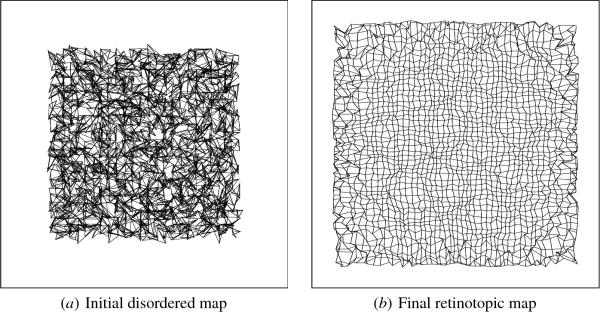
Fig. 4.8. Self-organization of the retinotopic map. The center of gravity of the afferent weights of every third neuron in the 142 × 142 V1 is projected onto the retinal space (represented by the square outline). As in Figure 3.6, each center is connected to those of the four neighboring neurons by a line, representing the topographical organization of the map. Initially, the anatomical RF centers were slightly scattered topographically and the weight values were random (a). The map is contracted because the receptive fields were initially mapped to the central portion of the retina so that each neuron has full RFs (Figure A.1). As self-organization progresses, the map unfolds to form a regular retinotopic map (b). The map expands slightly during this process, because neurons near the edge become tuned to the peripheral regions of the input space (Figure 4.7a). The map does not fill the input space entirely, because the center of gravity will always be located slightly inside the space. These results show that LISSOM can learn retinotopy like SOM does, but using mechanisms more close to those in biology.