Click on the image to see a PDF version (for zooming in)

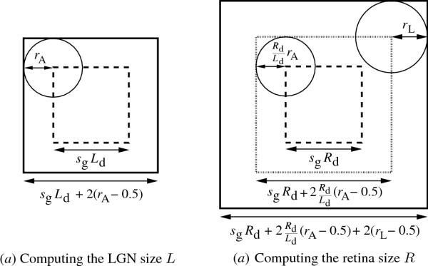
Fig. A.1. Mapping between neural sheets in LISSOM. In computing the LGN size L and the retina size R (Table A.2), a buffer area is added around the lower level sheet so that all neurons at the higher level have complete receptive fields. (a) In the mapping from LGN to V1, the outer square represents the LGN sheet, the dashed area maps point-for-point to V1, and the circle represents the receptive field of the top left V1 neuron. For instance, if s_g = 8 and L_d = 24, the dashed line encloses an area of 192 × 192 LGN units (8 × 24 = 192). This area is extended on all sides by r_A - 0.5 units to make sure that all V1 neurons have complete receptive fields. Thus, the LGN contains 204 × 204 neurons in total (192 + 2 × 6 = 204). (b) The mapping from retina to V1 is formed analogously, by extending the buffering down one more level. The outer square represents the retina, the dotted area maps point-for-point to the LGN, and the dashed area maps point-for-point to V1. The circle on the right shows the receptive field of the top right LGN neuron and the circle on the left represents the receptive field of the top left V1 neuron, with its radius expressed in retinal units (hence the factor R_d / L_d). For example, if R_d = 48, the dashed area is s_g R_d = 8 × 48 = 384 retinal units wide and the dotted area 384 + 2 × 48/24 × 6 = 408 retinal units wide. For an LGN 24 radius of r_L = 16.5, the full retina therefore consists of 440 × 440 neurons (384 + 2 × 48/24 × 6 + 2 × 16 = 440).