Click on the image to see a PDF version (for zooming in)

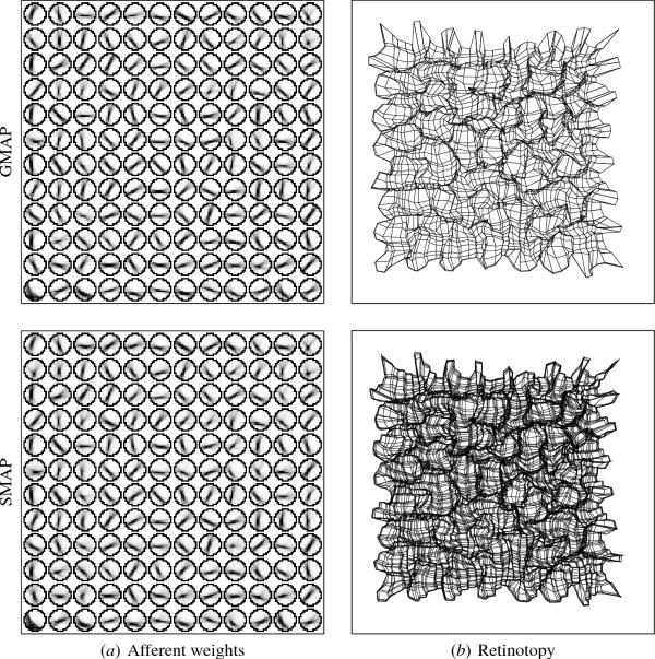
Fig. 11.3. Self-organized afferent weights and retinotopic organization. In (a), the afferent weight matrices of corresponding sample neurons in SMAP and GMAP are plotted (in gray scale as in Figure 6.4, organized as in Figure 5.8a): In SMAP, every fourth neuron horizontally and vertically is shown, and in GMAP, every tenth neuron. Both maps saw the same inputs during training, and due to the intracolumnar connections they developed matching orientation preferences. Since the ON/OFF channels in the LGN were bypassed in this simulation, the receptive fields are all unimodal. However, they display the same properties as the orientation model in Section 5.3: Most neurons are highly selective for orientation, and neurons near discontinuities are unselective. In (b), the center of gravity of the afferent weights of each neuron in the network are plotted as a grid in retinal space (as in Figure 5.11). Although the two maps differ in size, the overall organization closely matches: Neurons in the same cortical column receive input from the same locations in the retinal space. The overall organization of the map is an evenly spaced grid with local distortions, as observed in biology and in the LISSOM orientation map (Figure 5.11; Das and Gilbert 1997). The preferences are sharper and the distortions wider than in the LISSOM simulations because more elongated input patterns were used during training.