Service Curve Method

 

In Section 1 we informally introduced the service curve model. In this section we apply this method to derive a closed form for a lower bound on the worst-case end-to-end delay for Connection 0 in Section 4 using the service curve method.. We first derive a closed form for an upper bound on the service curve for a FIFO server, and then apply this result to derive the upper bound on the worst-case end-to-end delay lower bound on the worst case delay.

Let be the input traffic function of Connection i at Server k and be the constraint function of input traffic , and let be the output traffic of Connection i at Server k and be the constraint function of output traffic .

 

The service curve can be used to effectively evaluate the end-to-end delay suffered by traffic, as described in the following theorem.

Consider Server k in Figure 3 serving n+1 connections. Let

and

 

Proof:

For any time t, the amount of data departing the server during [0,t) is , and is the time of the -th bit arrival at the server. Since the server uses a FIFO scheduling discipline, we know that bits of data from Connection i have departed the server during time interval [0,t). So

Therefore, by the definition, we know that if

then is a service curve of Connection i offered by Server k. Q.E.D

Let

 

and

 

The definition for service curve is very loose. For a connection, there are infinitely many functions that satisfy Inequality (C.26). For example, a function with zero value is a service curve by the definition. In the following, we define an approximation for the service curve of a FIFO server.

 

Proof:

For any , if for , let , we have that

On the other hand, let for all , it is easy to know that

and

Therefore, we have that

and

This is a contradiction to Lemma C.6. Q.E.D

Proof:

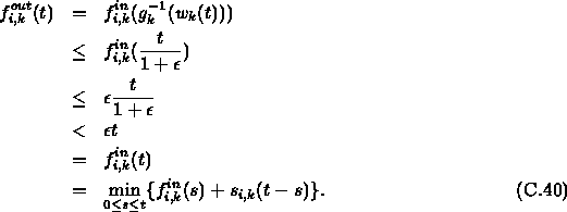
According to Theorem C.4, we have that . For , the maximum available service for Connection i during time interval [0,t) is . Therefore for all . Q.E.D

In order to use the above results, we need to accurately estimate the internal network traffic. Following Lemma C.6 gives a tight estimation about the constraint function of output traffic of each connection.

 

Proof:

Let be the time such that . Without loss of generality, we assume that for and , for . After time , we assume that for and , for . Since at time , the queue length of Server k is , according to FIFO scheduling discipline, during , the output traffic of Connection i is zero. But after time , the output traffic of Connection j ( ) is zero. Hence

and

Therefore we have that

Q.E.D

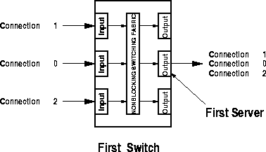
Now we can approximate the service curves offered by servers to Connection 0 in the example presented in Section 4.

Proof:

According to Theorem C.4, for k=1, we have

 

  

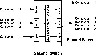
Figure 9: Connections at the First and the Second Server.

 

For k=2, we know that the traffic constraint functions for Connection 3 and Connection 4 are the same as . Furthermore, by Lemma C.6, the constraint function of Connection 2 is lower bounded by , where is the maximum queue length of the middle output port of the first switch when it only serves Connection 0 and Connection 1 and can be easy evaluated as

Substitute into , we have that . Therefore by Theorem C.4, we obtain that

 
Figure 10: Connections at the k-th switch.  

For k>2, similarly, we can obtain that

where is the maximum queue length of the middle output port of the (k-1)-th server when it only serves Connection 0, Connection (2k-3), and Connection (2k-4) and can be easy evaluated as

Therefore, we have

Q.E.D

According to Theorem C.4, network service curve of Connection 0 can be estimated as following:

Therefore