Due Wednesday, 10/27 at 23:59:59. You must work individually.
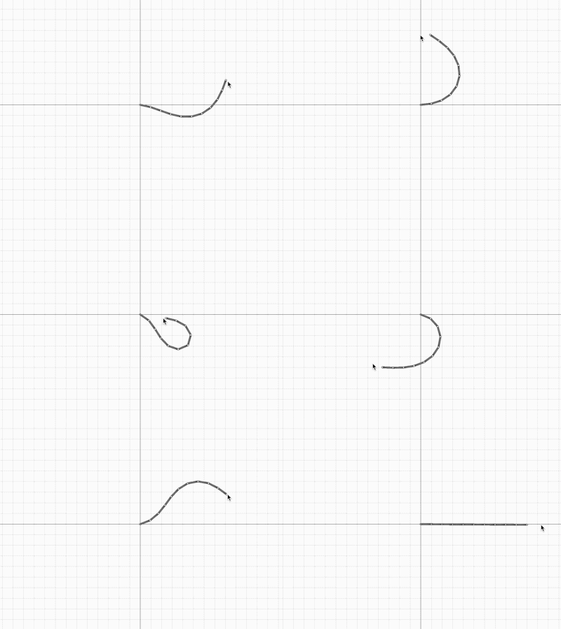
In this assignment, you will be implementing inverse kinematics with your own nonlinear solver:
Grades will be given out depending on how far you get along in the assignment. For example, if your program works with \(4\) links, then you will get full points for the \(1\)- and \(2\)-link tasks.
Here is an example with \(10\) links:

The best starting point is Lab 6. Implement forward kinematics fully before attempting inverse kinematics.
For quick reference, this is a listing of all the parameters to be used in the optimizers:
1e31e0iterMax: 10*n, where n is the number of linksalphaInit: 1e-4 (This is for \(n=10\). For other tasks, use 1e0).tol: 1e-3iterMax: 10*n, where n is the number of linkstol: 1e-3Note that the tolerance should be set to a relatively high value of 1e-3, since anything smaller will not make any visual difference. Also, as written above, the initial \(\alpha\) value may need to be bigger (e.g., 1e0) for \(1\)-, \(2\)-, and \(4\)-link tasks.
We will start slowly. First, we will solve inverse kinematics with only \(1\) joint using Gradient Descent with [Backtracking] Line Search (GDLS).

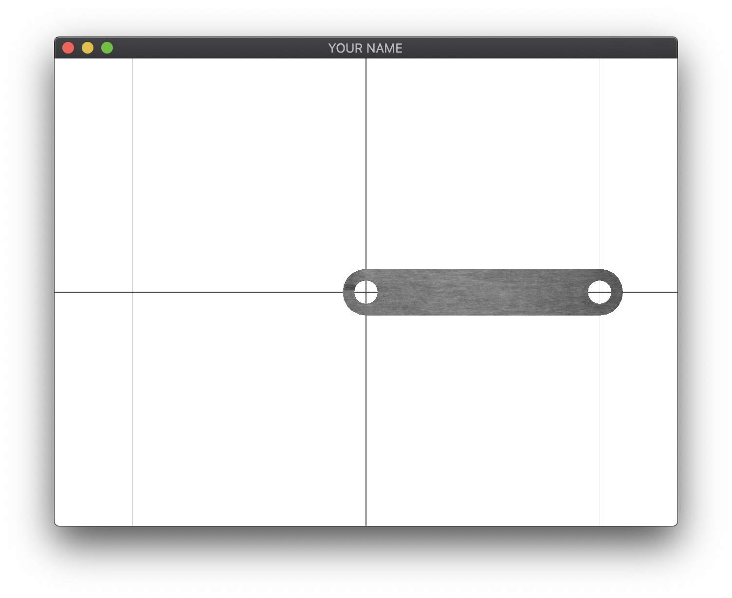
Each link is of length \(1.0\), so place an end-effector \(\vec{r}\) in the local coordinate space of the link: r = [1 0]'. Keep in mind that there should be a homogeneous coordinate of \(1\) for this point. In your code, it is a good idea to use Vector3d instead of Vector2d and explicitly store the homogeneous coordinate. On the other hand, it is ok to drop the homogeneous coordinate from \(\vec{p}\), \(\vec{p}'\), and \(\vec{p}''\).
The world-space position, \(\vec{p}\), of the end-effector and its derivatives are:
\[ \displaylines{ \vec{p}(\theta) = T R(\theta) \vec{r}\\ \vec{p}'(\theta) = T R'(\theta) \vec{r}\\ \vec{p}''(\theta) = T R''(\theta) \vec{r}, } \]
where \(R(\theta)\) is the usual rotation matrix about the Z-axis:
\[ \displaylines{ R(\theta) = \begin{pmatrix} \cos(\theta) & -\sin(\theta) & 0\\ \sin(\theta) & \cos(\theta) & 0\\ 0 & 0 & 1 \end{pmatrix}\\ R'(\theta) = \begin{pmatrix} -\sin(\theta) & -\cos(\theta) & 0\\ \cos(\theta) & -\sin(\theta) & 0\\ 0 & 0 & 0 \end{pmatrix}\\ R''(\theta) = \begin{pmatrix} -\cos(\theta) & \sin(\theta) & 0\\ -\sin(\theta) & -\cos(\theta) & 0\\ 0 & 0 & 0 \end{pmatrix}. } \]
The second derivative, \(\vec{p}''(\theta)\) and \(R''(\theta)\), will not be needed until we use Newton’s Method.
In the original rest state (figure above), the numerical values for the \(1\)-link system are (homogeneous coordinate not shown):
\[ \displaylines{ \vec{p}(\theta) = \begin{pmatrix} 1 \\ 0 \end{pmatrix}\\ \vec{p}'(\theta) = \begin{pmatrix} 0 \\ 1 \end{pmatrix}\\ \vec{p}''(\theta) = \begin{pmatrix} -1 \\ 0 \end{pmatrix}. } \]
For Gradient Descent, with or without line search, we need the objective function value \(f(\theta)\) and its gradient, \(\vec{g}(\theta)\). (We don’t need the Hessian, \(H(\theta),\) until we get to Newton’s Method.) The objective value is
\[ \displaylines{ f(\theta) = \frac{1}{2} w_\text{tar} \Delta \vec{p}^\top \Delta \vec{p} + \frac{1}{2} w_\text{reg} \Delta \theta^2\\ \Delta \vec{p} = \vec{p}(\theta) - \vec{p}_\text{target} \qquad\qquad\quad\;\;\,\\ \Delta \theta = \theta - \theta_\text{rest}. \qquad\qquad\qquad\quad\;\; } \]
The two weights, \(w_\text{tar}\) and \(w_\text{reg}\), can be set to arbitrary positive values, depending on the desired strength of the “targeting” energy and the “regularizer” energy.
You can use \(w_\text{tar} = 1e3\) and \(w_\text{reg} = 1e0\) for all tasks of this assignment.
The gradient is a scalar for this \(1\)-link task:
\[ g(\theta) = w_\text{tar} \Delta \vec{p}^\top \vec{p}' + w_\text{reg} \Delta \theta. \]
The Hessian (not needed yet) is also a scalar for this \(1\)-link task:
\[ H(\theta) = w_\text{tar} (\vec{p}'^\top \vec{p}' + \Delta \vec{p}^\top \vec{p}'') + w_\text{reg}. \]
With the initial angle set to \(\theta = 0\), and with the goal position set to \(\vec{p}_\text{goal} = (0 \; 1)^\top\), you should get the following values:
\[ f(\theta) = 1000, \quad g(\theta) = -1000, \quad H(\theta) = 1. \]
Run GDLS for a few iterations (e.g., 10-50 iterations). The returned answer should be close to, but not exactly \(\theta = \pi/2\). The exact answer will differ somewhat, based on the exact implementation of GDLS.
User Interface
Now let the end-effector goal be driven by the mouse. Set up your code so that pressing the space bar toggles between forward kinematics and inverse kinematics.
. and , keys.r key should reset all the angles to 0.0.The answer returned by GDLS will be visibly wrong because GDLS converges slowly. Therefore, we’re going to run a few iterations of NM to improve the answer. However, we must be careful since Newton’s Method can often get stuck in a local minimum. We’re going to take the following approach:
This ensures that we use the result of NM only if it improved upon the result of GDLS. With the combined approach above, you should get a visibly better result within a few Newton iterations.
Please output to the console the number of iterations taken by GDLS and by NM.
Next, we’re going to write a version that supports \(2\) links. If you’re feeling ambitious, you can skip to the \(4\)-link or the \(n\)-link tasks.
With two links, the minimization variable, \(\vec{\theta}\), is now a vector. The world-space position, \(\vec{p}\), of the end-effector is:
\[ \vec{p}(\vec\theta) = T_0 R_0(\theta_0) T_1 R_1(\theta_1) \vec{r}. \]
The derivatives are no longer scalars. The first derivative is a matrix of size \(2 \times 2\) (or \(1 \times 2\) block vector of \(2 \times 1\) vectors):
\[ \displaylines{ P'(\vec\theta) = \begin{pmatrix} \vec{p}'_0 & \vec{p}'_1 \end{pmatrix}\\ \vec{p}'_0 = T_0 R'_0(\theta_0) T_1 R_1(\theta_1) \vec{r}\\ \vec{p}'_1 = T_0 R_0(\theta_0) T_1 R'_1(\theta_1) \vec{r}. } \]
The second derivative is a matrix of size \(4 \times 2\) (or \(2 \times 2\) block matrix of \(2 \times 1\) vectors):
\[ \displaylines{ P''(\vec\theta) = \begin{pmatrix} \vec{p}''_{00} & \vec{p}''_{01} \\ \vec{p}''_{10} & \vec{p}''_{11} \end{pmatrix}\\ \vec{p}''_{00} = T_0 R''_0(\theta_0) T_1 R_1(\theta_1) \vec{r}\\ \vec{p}''_{01} = T_0 R'_0(\theta_0) T_1 R'_1(\theta_1) \vec{r}\\ \vec{p}''_{10} = T_0 R'_0(\theta_0) T_1 R'_1(\theta_1) \vec{r}\\ \vec{p}''_{11} = T_0 R_0(\theta_0) T_1 R''_1(\theta_1) \vec{r}. } \]
The objective function, \(f(\vec\theta)\), is still a scalar. In fact, the objective function for an optimization problem always returns a scalar. Compared to the \(1\)-link case, the only difference is that \(\Delta \vec\theta\), the deviation of the current joint angles from the rest joint angles, is now a vector. Therefore, instead of squaring this difference, we take the dot product by itself (i.e., transpose and multiply).
\[ f(\vec\theta) = \frac{1}{2} w_\text{tar} \Delta \vec{p}^\top \Delta \vec{p} + \frac{1}{2} w_\text{reg} \Delta \vec\theta^\top \Delta \vec\theta. \]
Now the gradient is a vector:
\[ \displaylines{ \vec{g}(\vec\theta) = w_\text{tar} \Delta \vec{p}^\top P' + w_\text{reg} \Delta \vec\theta \qquad\qquad\quad\;\\ = w_\text{tar} \begin{pmatrix} \Delta \vec{p}^\top \vec{p}'_0\\ \Delta \vec{p}^\top \vec{p}'_1 \end{pmatrix} + w_\text{reg} \begin{pmatrix} \Delta \theta_0\\ \Delta \theta_1 \end{pmatrix}. } \]
And the Hessian is a matrix:
\[ \displaylines{ H(\vec\theta) = w_\text{tar} (P'^\top P' + \Delta \vec{p}^\top \odot P'') + w_\text{reg} I \qquad\qquad\qquad\qquad\qquad\qquad\qquad\quad\;\,\\ = w_\text{tar} \left( \begin{pmatrix} \vec{p}_0^{'\top} \vec{p}'_0 & \vec{p}_0^{'\top} \vec{p}'_1\\ \vec{p}_1^{'\top} \vec{p}'_0 & \vec{p}_1^{'\top} \vec{p}'_1 \end{pmatrix} + \begin{pmatrix} \Delta \vec{p}^\top \vec{p}''_{00} & \Delta \vec{p}^\top \vec{p}''_{01}\\ \Delta \vec{p}^\top \vec{p}''_{10} & \Delta \vec{p}^\top \vec{p}''_{11} \end{pmatrix} \right) + w_\text{reg} \begin{pmatrix} 1 & 0\\ 0 & 1 \end{pmatrix}. } \]
The \(\odot\) symbol above is used to mean that \(\Delta \vec{p}\) is dotted with each vector element of \(P''\).
With the initial angle set to \(\vec{\theta} = (0 \; 0)^\top\), and with the goal position set to \(\vec{p}_\text{goal} = (1 \; 1)^\top\), you should get the following values:
\[ \vec{p}(\vec{\theta}) = \begin{pmatrix} 2\\ 0 \end{pmatrix}, \quad P'(\vec{\theta}) = \begin{pmatrix} 0 & 0\\ 2 & 1\\ \end{pmatrix}, \quad P''(\vec{\theta}) = \begin{pmatrix} -2 & -1\\ 0 & 0\\ -1 & -1\\ 0 & 0 \end{pmatrix}, \quad f(\vec{\theta}) = 1000, \quad \vec{g}(\vec{\theta}) = \begin{pmatrix} -2000\\ -1000 \end{pmatrix}, \quad H(\vec{\theta}) = \begin{pmatrix} 2001 & 1000\\ 1000 & 1 \end{pmatrix}. \]
Wrapping \(\theta\)
Since the minimization variables are joint angles, these variables may wrap around beyond (clockwise or counterclockwise) many times over. To prevent this, wrap the angles to be between \(-\pi\) and \(+\pi\) after each call to GDLS or NM with the following pseudocode:
while angle > pi
    angle -= 2*pi
while angle < -pi
    angle += 2*pi
Debugging the Derivatives
One of the biggest sources of bugs is the derivatives, so it is helpful to have a routine that tests them against finite differences. To test the gradient vector, use the following code inside the main loop of GDLS:
double e = 1e-7;
VectorXd g_(n);
for(int i = 0; i < n; ++i) {
    VectorXd theta_ = theta;
    theta_(i) += e;
    double f_ = objective->evalObjective(theta_);
    g_(i) = (f_ - f)/e;
}
cout << "g: " << (g_ - g).norm() << endl;
The finite differenced version of the gradient, g_, should closely match the analytical version of the gradient, g (at least within 1e-3 or so).
To test the Hessian matrix, use the following code inside the main loop of NM:
double e = 1e-7;
MatrixXd H_(n, n);
for(int i = 0; i < n; ++i) {
    VectorXd theta_ = theta;
    theta_(i) += e;
    VectorXd g_(n);
    objective->evalObjective(theta_, g_);
    H_.col(i) = (g_ - g)/e;
}
cout << "H: " << (H_ - H).norm() << endl;
The finite differenced version of the Hessian, H_, should closely match the analytical version of the Hessian, H.
In this task, you’re going to hard code a \(4\)-link system, which follows the same steps as in the \(2\)-link system. If you’re feeling ambitious, you can skip this task and go straight to the \(n\)-link system.
If you skipped \(2\)-link IK, make sure to read the Wrapping and Debugging sections.
The minimization variable is now \(\vec\theta = (\theta_0 \; \theta_1 \; \theta_2 \; \theta_3)^\top\). The world-space position, \(\vec{p}\), of the end-effector is:
\[ \vec{p}(\vec\theta) = T_0 R_0(\theta_0) T_1 R_1(\theta_1) T_2 R_2(\theta_2) T_3 R_3(\theta_3) \vec{r}. \]
The first derivative is a matrix of size \(2 \times 4\) (or \(1 \times 4\) block vector of \(2 \times 1\) vectors):
\[ \displaylines{ P'(\vec\theta) = \begin{pmatrix} \vec{p}'_0 & \vec{p}'_1 & \vec{p}'_2 & \vec{p}'_3 \end{pmatrix}\\ \vec{p}'_0 = T_0 R'_0(\theta_0) T_1 R_1(\theta_1) T_2 R_2(\theta_2) T_3 R_3(\theta_3) \vec{r}\\ \vec{p}'_1 = T_0 R_0(\theta_0) T_1 R'_1(\theta_1) T_2 R_2(\theta_2) T_3 R_3(\theta_3) \vec{r}\\ \vec{p}'_2 = T_0 R_0(\theta_0) T_1 R_1(\theta_1) T_2 R'_2(\theta_2) T_3 R_3(\theta_3) \vec{r}\\ \vec{p}'_3 = T_0 R_0(\theta_0) T_1 R_1(\theta_1) T_2 R_2(\theta_2) T_3 R'_3(\theta_3) \vec{r}. } \]
The second derivative is a matrix of size \(8 \times 4\) (or \(4 \times 4\) block vector of \(2 \times 1\) vectors):
\[ \displaylines{ P''(\vec\theta) = \begin{pmatrix} \vec{p}''_{00} & \vec{p}''_{01} & \vec{p}''_{02} & \vec{p}''_{03}\\ \vec{p}''_{10} & \vec{p}''_{11} & \vec{p}''_{12} & \vec{p}''_{13}\\ \vec{p}''_{20} & \vec{p}''_{21} & \vec{p}''_{22} & \vec{p}''_{23}\\ \vec{p}''_{30} & \vec{p}''_{31} & \vec{p}''_{32} & \vec{p}''_{33} \end{pmatrix}\\ \vec{p}''_{00} = T_0 R''_0(\theta_0) T_1 R_1(\theta_1) T_2 R_2(\theta_2) T_3 R_3(\theta_3) \vec{r}\\ \vec{p}''_{01} = T_0 R'_0(\theta_0) T_1 R'_1(\theta_1) T_2 R_2(\theta_2) T_3 R_3(\theta_3) \vec{r}\\ \vec{p}''_{02} = T_0 R'_0(\theta_0) T_1 R_1(\theta_1) T_2 R'_2(\theta_2) T_3 R_3(\theta_3) \vec{r}\\ \vdots\\ \vec{p}''_{32} = T_0 R_0(\theta_0) T_1 R_1(\theta_1) T_2 R'_2(\theta_2) T_3 R'_3(\theta_3) \vec{r}\\ \vec{p}''_{33} = T_0 R_0(\theta_0) T_1 R_1(\theta_1) T_2 R_2(\theta_2) T_3 R''_3(\theta_3) \vec{r}. } \]
The scalar objective function is:
\[ f(\vec\theta) = \frac{1}{2} w_\text{tar} \Delta \vec{p}^\top \Delta \vec{p} + \frac{1}{2} w_\text{reg} \Delta \vec\theta^\top \Delta \vec\theta. \]
The gradient, expressed as a column vector is:
\[ \displaylines{ \vec{g}(\vec\theta) = w_\text{tar} \Delta \vec{p}^\top P' + w_\text{reg} \Delta \vec\theta \qquad\qquad\quad\quad\\ = w_\text{tar} \begin{pmatrix} \Delta \vec{p}^\top \vec{p}'_0\\ \Delta \vec{p}^\top \vec{p}'_1\\ \Delta \vec{p}^\top \vec{p}'_2\\ \Delta \vec{p}^\top \vec{p}'_3 \end{pmatrix} + w_\text{reg} \begin{pmatrix} \Delta \theta_0\\ \Delta \theta_1\\ \Delta \theta_2\\ \Delta \theta_3 \end{pmatrix}. } \]
And the Hessian is a matrix:
\[ \displaylines{ H(\vec\theta) = w_\text{tar} (P'^\top P' + \Delta \vec{p}^\top \odot P'') + w_\text{reg} I \qquad\qquad\qquad\qquad\qquad\qquad\qquad\qquad\qquad\qquad\qquad\qquad\qquad\qquad\qquad\qquad\qquad\quad\\ = w_\text{tar} \left( \begin{pmatrix} \vec{p}_0^{'\top} \vec{p}'_0 & \vec{p}_0^{'\top} \vec{p}'_1 & \vec{p}_0^{'\top} \vec{p}'_2 & \vec{p}_0^{'\top} \vec{p}'_3\\ \vec{p}_1^{'\top} \vec{p}'_0 & \vec{p}_1^{'\top} \vec{p}'_1 & \vec{p}_1^{'\top} \vec{p}'_2 & \vec{p}_1^{'\top} \vec{p}'_3\\ \vec{p}_2^{'\top} \vec{p}'_0 & \vec{p}_2^{'\top} \vec{p}'_1 & \vec{p}_2^{'\top} \vec{p}'_2 & \vec{p}_2^{'\top} \vec{p}'_3\\ \vec{p}_3^{'\top} \vec{p}'_0 & \vec{p}_3^{'\top} \vec{p}'_1 & \vec{p}_3^{'\top} \vec{p}'_2 & \vec{p}_3^{'\top} \vec{p}'_3 \end{pmatrix} + \begin{pmatrix} \Delta \vec{p}^\top \vec{p}''_{00} & \Delta \vec{p}^\top \vec{p}''_{01} & \Delta \vec{p}^\top \vec{p}''_{02} & \Delta \vec{p}^\top \vec{p}''_{03}\\ \Delta \vec{p}^\top \vec{p}''_{10} & \Delta \vec{p}^\top \vec{p}''_{11} & \Delta \vec{p}^\top \vec{p}''_{12} & \Delta \vec{p}^\top \vec{p}''_{13}\\ \Delta \vec{p}^\top \vec{p}''_{20} & \Delta \vec{p}^\top \vec{p}''_{21} & \Delta \vec{p}^\top \vec{p}''_{22} & \Delta \vec{p}^\top \vec{p}''_{23}\\ \Delta \vec{p}^\top \vec{p}''_{30} & \Delta \vec{p}^\top \vec{p}''_{31} & \Delta \vec{p}^\top \vec{p}''_{32} & \Delta \vec{p}^\top \vec{p}''_{33} \end{pmatrix} \right) + w_\text{reg} \begin{pmatrix} 1 & 0 & 0 & 0\\ 0 & 1 & 0 & 0\\ 0 & 0 & 1 & 0\\ 0 & 0 & 0 & 1 \end{pmatrix}. } \]
The \(\odot\) symbol above is used to mean that \(\Delta \vec{p}\) is dotted with each vector element of \(P''\).
With the initial angle set to \(\vec{\theta} = (0 \; 0 \; 0 \; 0)^\top\), and with the goal position set to \(\vec{p}_\text{goal} = (3 \; 1)^\top\), you should get the following values:
\[ \vec{p}(\vec{\theta}) = \begin{pmatrix} 4\\ 0 \end{pmatrix}, \quad P'(\vec{\theta}) = \begin{pmatrix} 0 & 0 & 0 & 0\\ 4 & 3 & 2 & 1 \end{pmatrix}, \quad P''(\vec{\theta}) = \begin{pmatrix} -4 & -3 & -2 & -1\\ 0 & 0 & 0 & 0\\ -3 & -3 & -2 & -1\\ 0 & 0 & 0 & 0\\ -2 & -2 & -2 & -1\\ 0 & 0 & 0 & 0\\ -1 & -1 & -1 & -1\\ 0 & 0 & 0 & 0 \end{pmatrix}, \quad f(\vec{\theta}) = 1000, \quad \vec{g}(\vec{\theta}) = \begin{pmatrix} -4000\\ -3000\\ -2000\\ -1000 \end{pmatrix}, \quad H(\vec{\theta}) = \begin{pmatrix} 12001 & 9000 & 6000 & 3000\\ 9000 & 6001 & 4000 & 2000\\ 6000 & 4000 & 2001 & 1000\\ 3000 & 2000 & 1000 & 1 \end{pmatrix}. \]
Convert your code to support an arbitrary number of links. Note that as you increase \(n\), the code will get slower and slower. Make sure to run your code in release mode. It is recommended that you first work on GDLS and then NM.
If you skipped \(2\)-link IK, make sure to read the Wrapping and Debugging sections.
Total: 100 points
You can skip \(1\)-, \(2\)-, and \(4\)-link IK and go straight to \(n\)-link IK. Grades for lower tasks will be automatically given if the higher task is completed.
Failing to follow these points may decrease your “general execution” score.
Please output to the console the number of iterations taken by GDLS and by NM.
If you’re using Mac/Linux, make sure that your code compiles and runs by typing:
> mkdir build
> cd build
> cmake ..
> make
> ./A4 <RESOURCE DIR>
If you’re using Windows, make sure your code builds using the steps described in Lab 0.
(*.~), or object files (*.o). You should hand in the minimum set of files you need to compile plus the README file. Your “resources” directory should only contain your GLSL files.USERNAME.zip (e.g., sueda.zip). The zip file should extract everything into a folder named USERNAME/ (e.g. sueda/).
src/, resources/, CMakeLists.txt, and your README file to the USERNAME/ directory..zip format (not .gz, .7z, .rar, etc.).