Click on the image to see a PDF version (for zooming in)

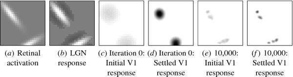
Fig. 5.6. Example input and response. A sample input on the retina, the LGN response, and the initial and settled cortical response before and after training are shown as in Figure 4.4, except the padding in retina and LGN is omitted so that all plots represent the same retinal area. To train the orientation map, two oriented Gaussians were drawn with random orientations and random, spatially separated locations on the retina (a). As discussed in Appendix A.4, while more than two spots could be used, they are too large to be distributed uniformly on the small retina. The LGN responses are plotted in (b) by subtracting the OFF cell responses from the ON. The LGN responds strongly to the edges of the oriented Gaussians. Initially, the responses of the V1 map are similar for all orientations (c and d). After 10,000 input presentations, the V1 response extends along the orientation of the stimulus, and is patchy because neurons that prefer similar positions but different orientations do not respond (e and f ). An animated demo of the map response can be seen at ...