Click on the image to see a PDF version (for zooming in)

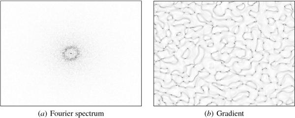
Fig. 5.1. Fourier spectrum and gradient of the macaque orientation map. Plot (a) shows the two-dimensional Fourier spectrum of the map in Figure 2.4, calculated using methods described by Erwin et al. (1995) on orientation map data from Blasdel (1992b). In this and subsequent Fourier spectrum figures, the center represents the DC component and the midpoint of each edge 1/2 of the highest possible spatial frequency of the image horizontally and vertically (i.e. the Nyquist frequency; Cover and Thomas 1991); the amplitude is represented in gray scale from white to black (low to high). As typically found in animal maps, the spectrum is ring shaped, indicating that the orientations repeat in all directions with a spatial frequency that corresponds to the radius of the ring. (b) The orientation gradient of the same map is plotted in gray scale from white to black (low to high; calculated from Blasdel 1992b as described in Appendix G.6). The high-gradient areas (dark ridges) correspond to fractures; the pinwheel centers are usually located at the ends of fractures. The gradient map makes the global arrangement of these features easy to characterize.