Click on the image to see a PDF version (for zooming in)

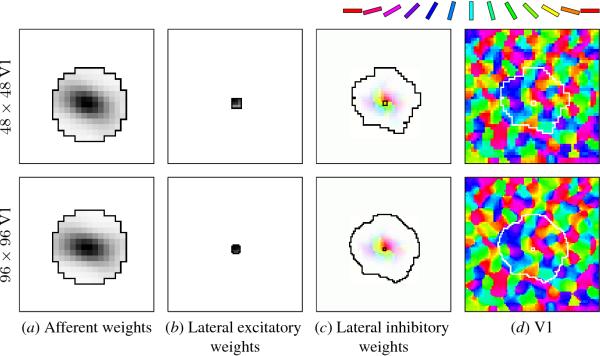
Fig. 15.6. Scaling cortical density in GLISSOM. In a single GLISSOM cortical density scaling step, a 48 × 48 V1 (top row) is expanded into a 96 × 96 V1 (bottom row) at iteration 10,000 out of a total of 20,000. Smaller scaling steps are usually more effective, but the large step makes the changes more obvious. A set of weights for one neuron in each network is shown in (a-c). At this point in training, the afferent and lateral connection profiles are still only weakly oriented, and lateral connections have not been pruned extensively (the jagged black outline in (c) shows the current connectivity). The orientation map for each network is shown in (d), with the inhibitory weights of the sample neuron overlaid in white outline. The orientation map measured from the scaled map is identical to that of the 48 × 48 network, except that it has twice the resolution. This network can then self-organize at the new density to represent finer detail.