Click on the image to see a PDF version (for zooming in)

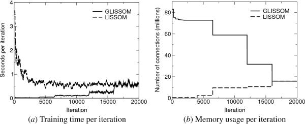
Fig. 15.4. Training time and memory usage in LISSOM vs. GLISSOM. Data are shown for a LISSOM network of 144 × 144 units and a GLISSOM network grown from 36 × 36 to 144 × 144 units as described in Section 15.4.2. (a) Each line shows a 20-point running average of the time spent in training for one iteration, with a data point measured every 10 iterations. Only training time is shown; times for initialization, plotting images, pruning, and scaling networks are not included. Computational requirements of LISSOM peak at the early iterations, falling as the excitatory radius (and thus the number of neurons activated by a given pattern) shrinks and as the neurons become more selective. In contrast, GLISSOM requires little computation time until the final iterations. Because the total training time is determined by the area under each curve, GLISSOM is much more efficient to train overall. (b) Each line shows the number of connections simulated at a given iteration. LISSOM's memory usage peaks at early iterations, decreasing at first in a series of small drops as the lateral excitatory radius shrinks, and then later in a few large drops as long-range inhibitory weights are pruned at iterations 6500, 12,000, and 16,000. Similar shrinking and pruning takes place in GLISSOM, while the network size is scaled up at iterations 4000, 6500, 12,000, and 16,000. Because the GLISSOM map starts out small, memory usage peaks much later, and remains bounded because connections are pruned as the network is grown. As a result, the peak number of connections (which determines the memory usage) in GLISSOM is as low as the smallest number of connections in LISSOM.