Click on the image to see a PDF version (for zooming in)

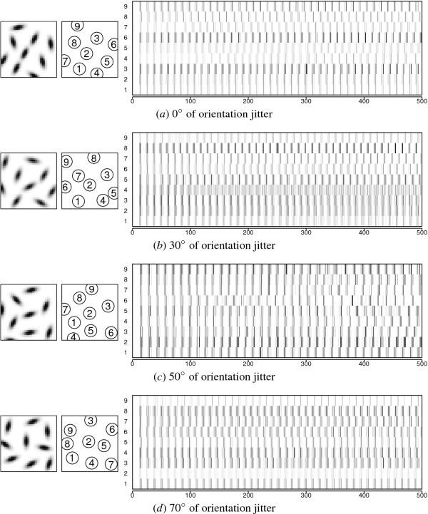
Fig. 13.6. Contour integration process with varying degrees of orientation jitter. In each subfigure, the input presented to the network is shown at left, the areas in GMAP where MUA was measured in the middle, and the resulting MUA plot at right. Each contour was composed of three contour elements, and embedded in a background of six randomly oriented elements. Each contour runs diagonally from lower left to top right with varying degrees of orientation jitter. The MUA of each area is plotted in gray scale from white (no neurons firing in the area at this time step) to black (all neurons firing). Time (i.e. simulation iteration) is on the x-axis and the y-axis consists of nine rows, each plotting the MUA of the area labeled with the row number. The three bottom rows (1 to 3) represent the MUAs of the salient contour, and the six top rows (4 to 9) the MUAs of the background elements. The contour is very strongly synchronized for 0^o and 30^o but relatively weakly synchronized for 50^o and 70^o of orientation jitter: The contours get harder to detect as the jitter increases. In all cases (a to d), the background MUAs are unsynchronized. A quantitative summary of these results is shown in Figure 13.7, and an animated demo can be seen at ...