Due Wednesday, 9/15 Friday, 9/17 at 23:59:59. You must work individually.
In this assignment, you will be creating a keyframed animation of a toy helicopter.
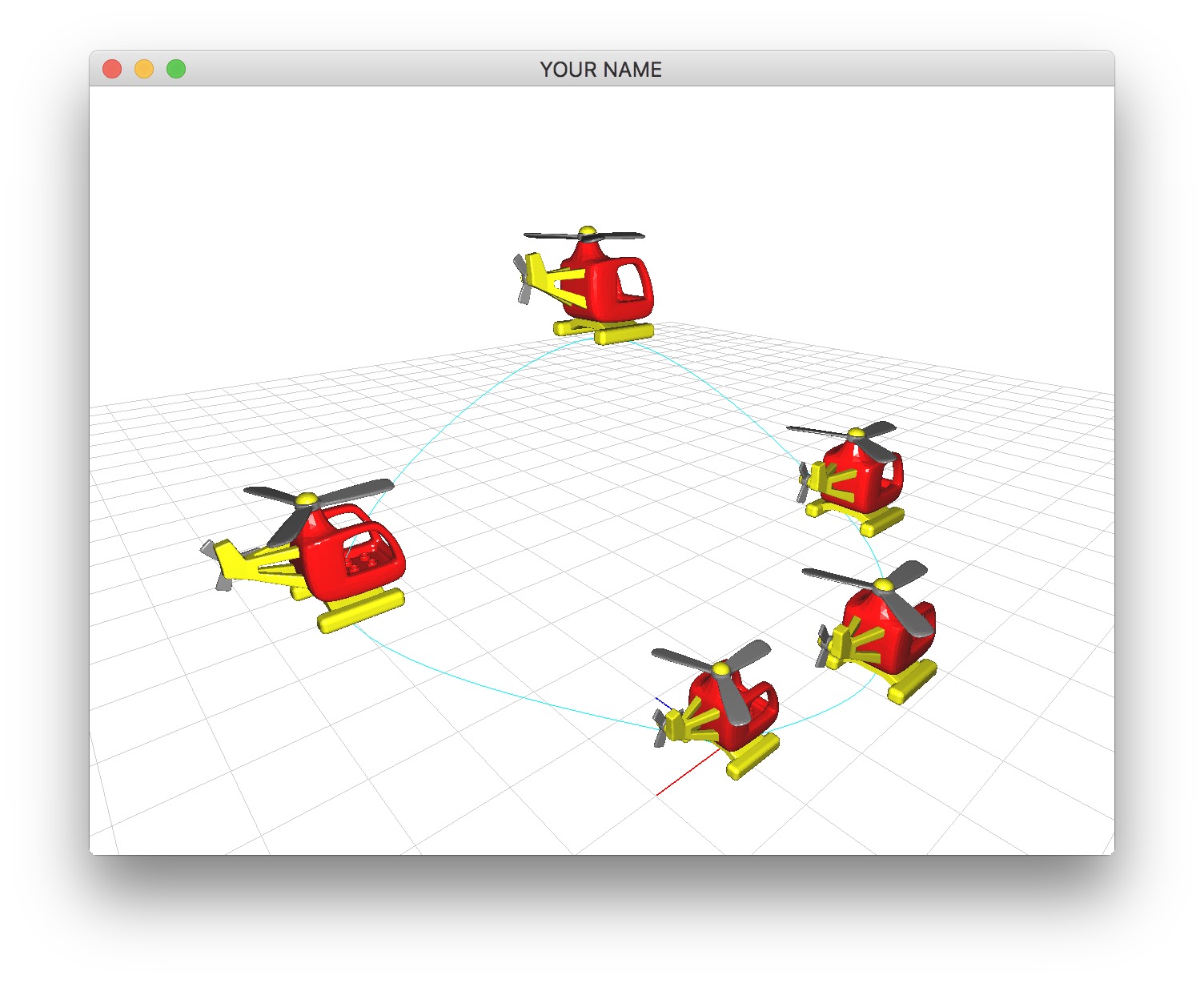
In this assignment, instead of interpolating between two keyframes like in Lab 2, you will be interpolating between many different keyframes. For example, in the figure above, there are 5 keyframes that we’re interpolating between.
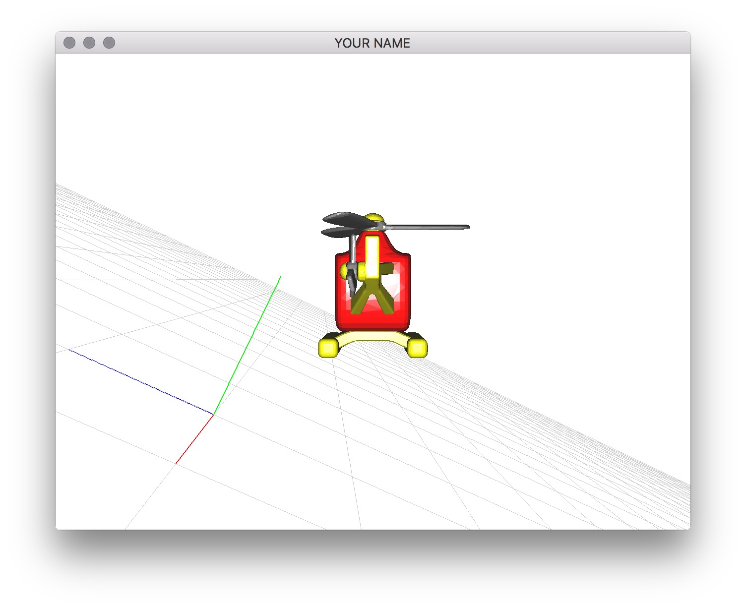
Download the skeleton code for the assignment. When you run the starter code, you should see one of the body meshes of the helicopter and the background grid. Keep in mind that you’re free to reorganize your code the way you see fit. It is a good idea to create several classes for this assignment. If you put everything in main.cpp, you will lose points.
Load and visualize the helicopter meshes. (These meshes are from Thingiverse.) There are 4 meshes — two for the body (shown in red and yellow here) and the two propellers (grey). If you want, you can change these colors, and/or write your own shader (e.g., Blinn-Phong).
Rotate the two propellers in place. The center of rotation of the \(1\)st propeller is at (0.0, 0.4819, 0.0), and the center of rotation of the \(2\)nd propeller is at (0.6228, 0.1179, 0.1365). In main.cpp’s render function, define a time variable: double t = glfwGetTime();, and rotate the propellers using this variable.
To start, define at least 5 positional keyframes. (We will deal with rotations later.) The helicopter should start and end at the origin. First, draw the helicopter at each keyframe. Use the k key to toggle on and off these keyframes.
Next, draw a Catmull-Rom spline curve that starts and ends at the origin. You will need to double up on the first and the last control points to make the curve start and end at the origin. This means that if you created 5 keyframes, then you’ll need 7 control points. Alternatively, You can implement a circular traversal of the control points to implement a closed loop. Once you finish this task, you should see the curve and a sequence of unrotated helicopters along the curve. By pressing the k key, you should be able to show/hide the curve and the positional keyframes.
Using the global time variable, t, draw an interpolated helicopter that translates along the curve (with no rotation). You can use this simple mapping between t and u:
float umax = #keyframes - 3;
float u = std::fmod(t, umax);
The variable umax is the largest valid value of u, which is #keyframes-3. This code ensures that u stays within the range 0 to umax. It should take umax seconds to complete the flight. The helicopter will not have a constant speed. You’ll fix this later.
NOTE The u computed with the pseudocode above is the “concatenated” u. Only the fractional part of this concatenated u should go into the vector \(\vec{u}\). In other words, the vector \(\vec{u}\) should only contain values between \(0\) and \(1\). The integral part of the concatenated u should be used to figure out which control points go into the G matrix. For example, if the concatenated u is \(0.9\), control points \(0\) through \(3\) should go into G, and \(0.9\) should go into \(\vec{u}\); if the concatenated u is \(1.1\), control points \(1\) through \(4\) should go into G, and \(0.1\) should go into \(\vec{u}\).
The control points should be defined in the init() function, rather than in the render() function, since these control points do not change.
Now you’re going to add rotation to the keyframes. Currently a keyframe consists only of a single glm::vec3 that represents the position. To this, you need to add a glm::quat that represents the rotation. This way, a keyframe can fully represent a rigid transform - position and orientation. This should be combined into a class that represents a keyframe. Once you have support for rotational keyframes, update your drawing code to use these new values. When you specify the rotation, you may want to use glm::angleAxis(...), since they are more intuitive geometrically. With rotations added, you should see something like the animation at the top of this page when you press the k key.
Now that you have the rotation keyframes, interpolate between them. There are sophisticated solutions for this problem, but for this assignment, you’re just going to use the same approach we used for positions. (Slerp is great for interpolating between two rotations, but if we use slerp between two successive rotations, then it will not look smooth across segments.) The steps are are analogous to how we interpolated positions. Before, we interpolated the position using four control points. Now we’re going to interpolate both positions and rotations using four control frames. The steps are:
u, use a Catmull-Rom spline to interpolate each component (x, y, z) of the position vector. (This is Task 2.)u, use the same Catmull-Rom spline to interpolate each component (x, y, z, w) of the rotation quaternion.Here is the glm code that does exactly that.
// Compute rotation
glm::vec4 uVec(1.0f, u, u*u, u*u*u);
// Fill G with rotation quaternion of the 4 control frames
...
glm::vec4 qVec = G * (B * uVec);
glm::quat q(qVec[3], qVec[0], qVec[1], qVec[2]); // Constructor argument order: (w, x, y, z)
glm::mat4 E = glm::mat4_cast(glm::normalize(q)); // Creates a rotation matrix

// Compute position
// Fill G with position vector of the 4 control frames
...
glm::vec3 p = G * (B * uVec);
E[3] = glm::vec4(p, 1.0f); // Puts the position into the last column
In the code above, the 4x4 matrix, G, is used twice. First, it is filled with the four quaternions that correspond to the current value of u, arranged column by column. Then, it is filled with the four positions that correspond to the same value of u, again arranged column by column. B is the 4x4 basis matrix for the Catmull-Rom spline. Note that the constructor for the glm quaternion class takes the ‘w’ component before the ‘x,y,z’ components. The 4x4 matrix, E, is the resulting rotation matrix. The last line is inserting the keyframe position into the last column of the matrix. This matrix can then be multiplied onto the matrix stack with a call to MV->multMatrix(). Once you complete this task, you should see the helicopter follow not only the position keyframes but also the rotation keyframes.
Remember to interpolate the rotations along the short route. Otherwise, you’ll see a weird ‘twirl’ between two keyframes. Each pair of successive quaternions must have a positive dot product. Go through the list of quaternions, and if the dot product of \(q_i\) and \(q_{i+1}\) is negative, then negate \(q_{i+1}\).
Finally, design an interesting animation that includes at least one loop or one roll or one interesting maneuver by specifying appropriate keyframes.
Because of the simple linearly relationship between t and u (defined in Task 2), the helicopter’s speed depends on the spacing of the keyframes. If two successive keyframes are close, then the helicopter will move slowly between them, and conversely, if two successive keyframes are far, the helicopter will move quickly between them. To fix this, you can no longer use the simple linear relationship between t and u. You need to replace it with arc-length parameterization. To do so, you need to apply two transformations:
t to s: time to arc lengths to u: arc length to spline parameterFor 2, follow the instructions from Lab 3 (Tasks 1 and 2). For 1, you can use a linear relationship:
float tNorm = std::fmod(t, tmax) / tmax;
float sNorm = tNorm;
float s = smax * sNorm;
Both tNorm and sNorm are normalized quantities, meaning they go from \(0\) to \(1\). tmax is the number of seconds you want the animation to take, and smax is the total length of the spline curve. Choose a good value for tmax, and put this in the README. The normalized time, tNorm, is 0 when t = 0, and 1 when t = tmax. Similarly, the normalized arc length, sNorm, is \(0\) when s = 0, and \(1\) when s = smax. Once this task is complete, the helicopter should move at a constant speed no matter where you place the control points, and it should complete its flight in tmax seconds. You should verify this by placing one of the keyframes far away. The helicopter should not move faster while moving to/from the keyframe.
Since the spline path does not change over time, the arc-length table should be defined in the init() function, rather than in the render() function.
Pressing the s key on the keyboard should swap between using and not using arc-length parameterization.
Implement time control so that the helicopter doesn’t simply move at a constant speed. To do this, you need to use a different mapping function between \(t\) and \(s\). For example, a simple ease in / ease out is achieved by a single cubic:
\[ s = −2t^3 + 3t^2 \]
Here, I’ve used s for sNorm and t for tNorm for brevity. First, implement this ease in/out curve. You should set up your code so that pressing the s key cycles between: no arc-length, with arc-length, and ease in/out.
Next, design some other interesting length/time curve. Some examples include:
At least one portion of the time curve must involve solving a 4x4 linear system. This can be done with glm as follows:
glm::mat4 A;
glm::vec4 b;
// Fill A and b
...
// Solve for x
glm::vec4 x = glm::inverse(A) * b;
A glm matrix can be filled in column by column: A[0] = glm::vec4(...);. (For bigger linear systems, use the Eigen library and use a stable linear solver.)
In the README, add a brief description of the time control function you used. By pressing the s key, you should be able to cycle between: no arc-length, with arc-length, ease in/out, and your custom function.
Make the camera be on the helicopter. Pressing the space bar should toggle this feature on/off. (Switch between using the mouse to control the camera and using the helicopter location to control the camera.) Remember that the “view” matrix is the inverse of the “camera” matrix. Set the camera matrix to be the helicopter’s current matrix (possibly with some offset), take the inverse, and use the resulting matrix as the first matrix on the matrix stack. You can also use the lookAt() function, but I think it is easier to use the matrix method.
Rather than using the linear approximation of arc length, use a 3-point Gaussian quadrature, as in Lab 3: Task 2.
k key.tmax seconds).s key should cycle between different time modes.init(), rather than in render().Total: 100 plus 10 bonus points.
Failing to follow these points may decrease your “general execution” score.
If you’re using Mac/Linux, make sure that your code compiles and runs by typing:
> mkdir build
> cd build
> cmake ..
> make
> ./A1 ../resources
If you’re using Windows, make sure your code builds using the steps described in Lab 0.
For this assignment, there should be only one argument.
tmax value from Task 3src/, resources/, CMakeLists.txt, and your readme file. The resources folder should contain all required input obj and GLSL files.(*.~), or object files (*.o).USERNAME.zip (e.g., sueda.zip). The zip file should extract everything into a folder named USERNAME/ (e.g. sueda/).
src/, resources/, CMakeLists.txt, and your README file to the USERNAME/ directory..zip format (not .gz, .7z, .rar, etc.).