In this lab, we’re going to draw cubic spline curves in OpenGL.
Please download the lab and go over the code.
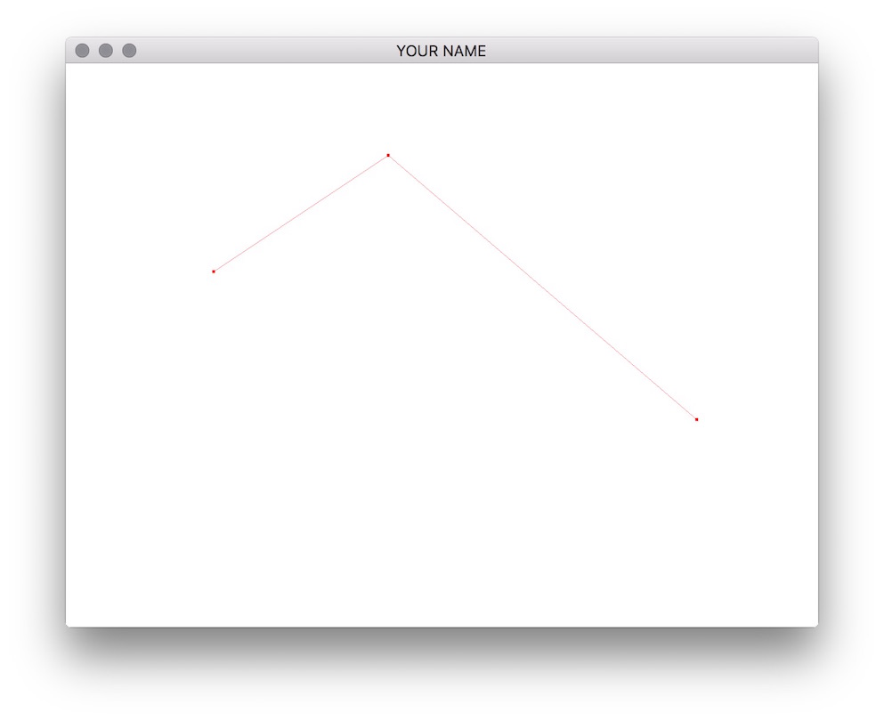
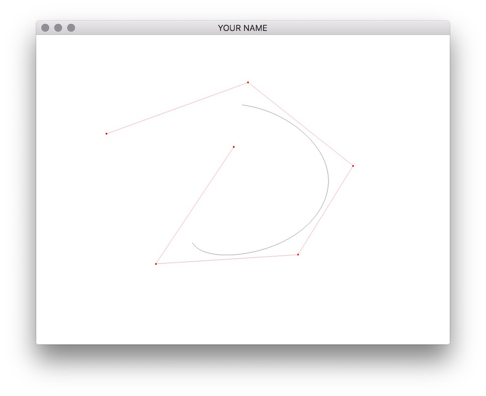
The code doesn’t draw any curves yet — it simply draws dots whenever you shift-click on the window. These are going to be the control points of the spline curve. These control points are in 3D. You can rotate the camera with the mouse. Pressing the L key will toggle on/off the connecting lines.
Look at line 183 of main.cpp. We’re using “immediate mode” (old-school OpenGL) for specifying the geometry and colors of the vertices. The basic syntax is:
glBegin(TYPE); // TYPE can be GL_POINTS, GL_LINE_STRIP, etc.
glColor3f(...);
glVertex3f(...);
glColor3f(...);
glVertex3f(...);
...
glEnd();
Everytime a vertex is specified with glVertex(), the last specified color will be used for that vertex.
Next, look at the vertex shader (simple_vert.glsl). With immediate mode, the vertex position is accessed with the built-in variable gl_Vertex, and the vertex color is accessed with the built-in variable gl_Color.
Using just the first four control points, draw a Bezier curve. The formula is given by the following matrix equation.
\[ \begin{aligned} p(u) &= G B \bar{u},\\ G &= \begin{pmatrix} x_0 & x_1 & x_2 & x_3\\ y_0 & y_1 & y_2 & y_3\\ z_0 & z_1 & z_2 & z_3 \end{pmatrix}, \quad B = \begin{pmatrix} 1 & -3 & 3 & -1\\ 0 & 3 & -6 & 3\\ 0 & 0 & 3 & -3\\ 0 & 0 & 0 & 1 \end{pmatrix}, \quad \bar{u} = \begin{pmatrix} 1\\ u\\ u^2\\ u^3 \end{pmatrix}. \end{aligned} \]
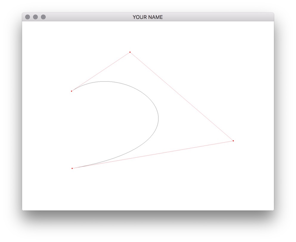
Here, \(p(u)\) is a 3x1 vector corresponding to the x, y, and z coordinates of the curve position at the parameter u. To draw the curve, the parameter u should go from 0 to 1. \(G\) is the geometry matrix, composed of the control point positions stored column by column. \(B\) is the spline basis matrix, which is different for each spline type.
With glm, you can create a 4x4 matrix using the built-in class glm::mat4 and a 4x1 vector using the built-in class glm::vec4. (If you declare using namespace glm;, you don’t need to say glm:: every time within that cpp file. Do not do this in an h file!) The G matrix is a 3x4 matrix, but you can use a 4x4 matrix and ignoring the bottom row. The basic flow should be something like this:
// Fill in B column by column
glm::mat4 B;
B[0] = glm::vec4(...);
...
// Fill in G column by column
glm::mat4 G;
G[0] = glm::vec4(cps[0], 0.0f);
G[1] = glm::vec4(cps[1], 0.0f);
G[2] = glm::vec4(cps[2], 0.0f);
G[3] = glm::vec4(cps[3], 0.0f);
...
glBegin(GL_LINE_STRIP);
for(...) {
    ...
    // Fill in uVec
    glm::vec4 uVec(1.0f, u, u*u, u*u*u);
    // Compute position at u
    glm::vec4 p = G*(B*uVec);
    ...
    glVertex3f(p.x, p.y, p.z);
}
glEnd();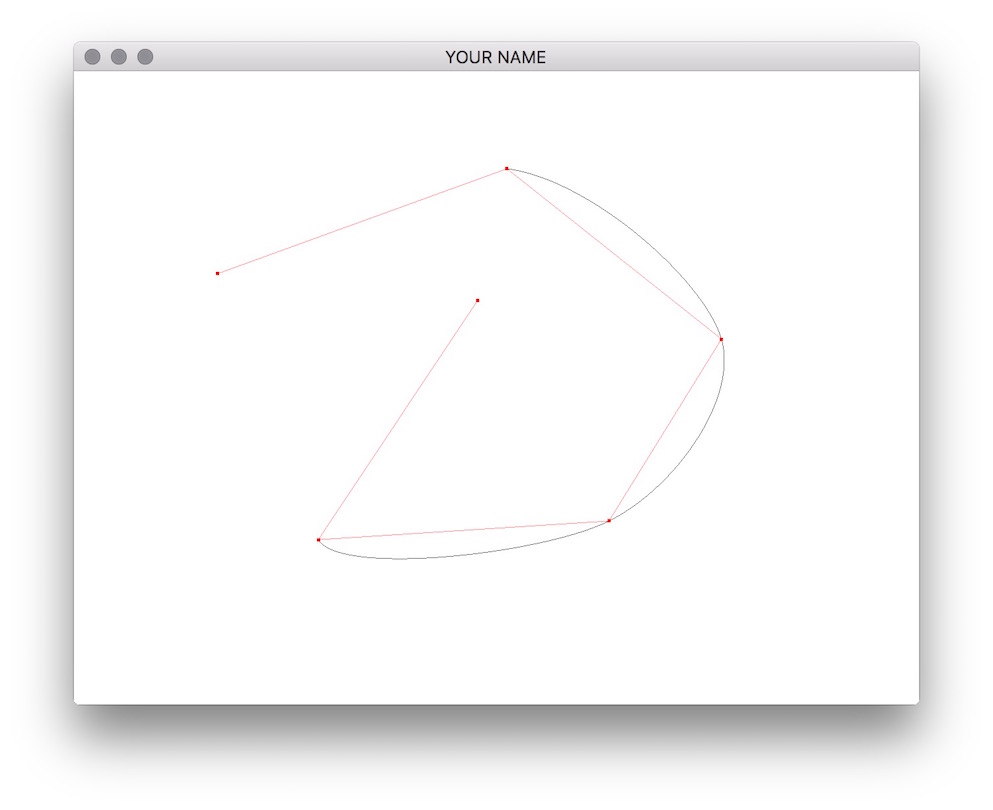
...There is a keyboard hook for the s key to change the spline type between Bezier splines, Catmull-Rom splines, and B-splines. Implement the remaining two. These two support any number (\(\ge 4\)) of control points, by connecting a sequence of cubic splines together. For example, if there are 6 control points, the control points 0, 1, 2, and 3 define the first segment, the control points 1, 2, 3, and 4 define the second segment, and finally, the control points 2, 3, 4 and 5 define the third segment.
The basis matrix for the Catmull-Rom spline is
\[ B = \frac{1}{2} \begin{pmatrix} 0 & -1 & 2 & -1\\ 2 & 0 & -5 & 3\\ 0 & 1 & 4 & -3\\ 0 & 0 & -1 & 1 \end{pmatrix}, \]
and the basis matrix for the B-spline is
\[ B = \frac{1}{6} \begin{pmatrix} 1 & -3 & 3 & -1\\ 4 & 0 & -6 & 3\\ 1 & 3 & 3 & -3\\ 0 & 0 & 0 & 1 \end{pmatrix}. \]
Note that Catmull-Rom splines are interpolating, whereas B-splines are approximating. Both are local in the sense that changing a control point only affects the curve locally and not globally.
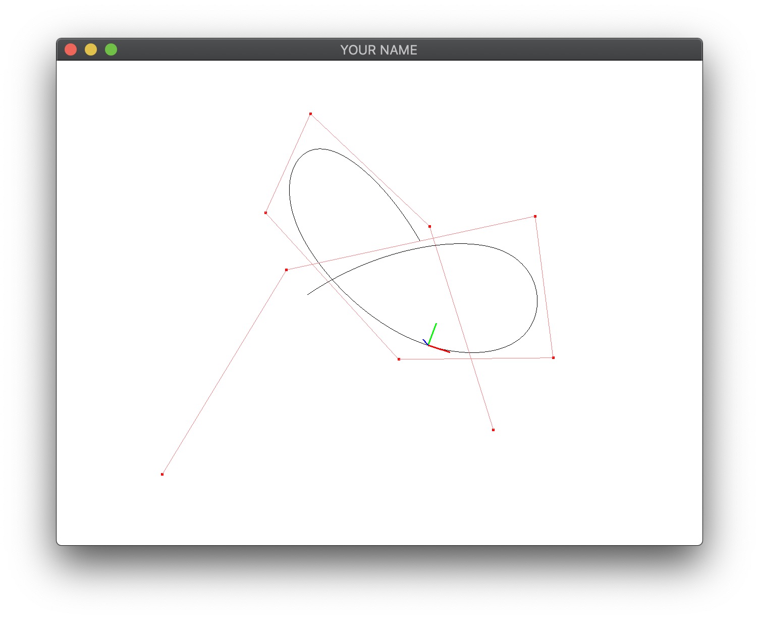
For the Catmull-Rom spline and the B-spline, draw the Frenet frame that moves along the curve (shown in red, green, and blue in the figure below). The tangent should be red, the normal should be green, and the binormal should be blue.
\[ \begin{aligned} p'(u) &= G B \bar{u}', \quad \bar{u}' = \begin{pmatrix} 0 & 1 & 2u & 3u^2\end{pmatrix}^T,\\ p''(u) &= G B \bar{u}'', \quad \bar{u}'' = \begin{pmatrix} 0 & 0 & 2 & 6u\end{pmatrix}^T,\\ T(u) &= \frac{p'(u)}{\|p'(u)\|},\\ B(u) &= \frac{p'(u) \times p''(u)}{\|p'(u) \times p''(u)\|},\\ N(u) &= B(u) \times T(u). \end{aligned} \]
The Frenet frame should travel along the curve using the global variable, t, which is incremented using a timer. You may need to scale the three vectors for display. You can use the following code to convert from t to u.
float kfloat;
float u = std::modf(std::fmod(t*0.5f, ncps-3.0f), &kfloat);
int k = (int)std::floor(kfloat);
This code ensures that u stays within the range 0 to 1, and that k is the appropriate index into the array of control points. The 0.5 implies that in when t changes by 1.0, u changes by 0.5, meaning the Frenet frame will take 2 seconds to go from one control point to the next.