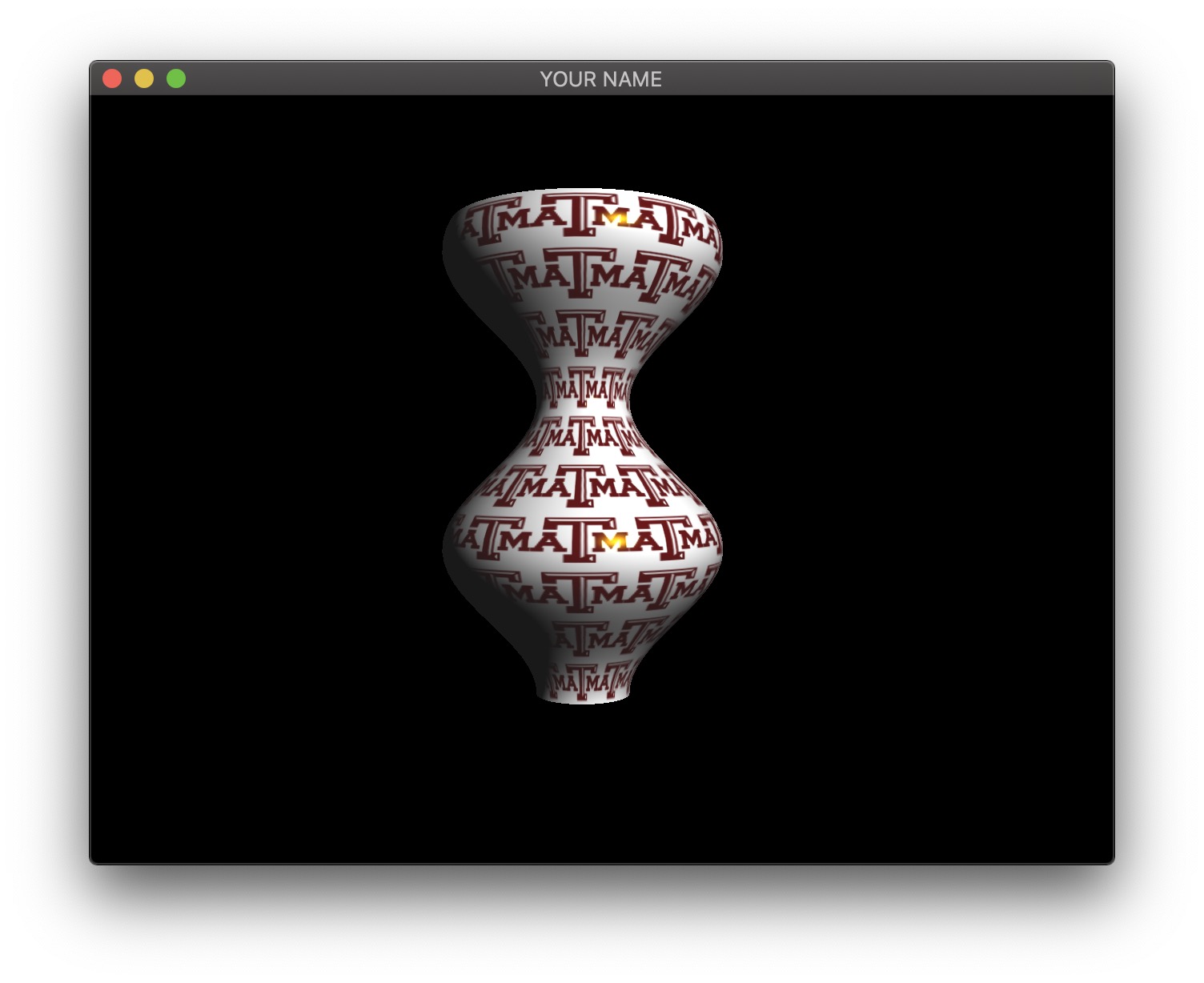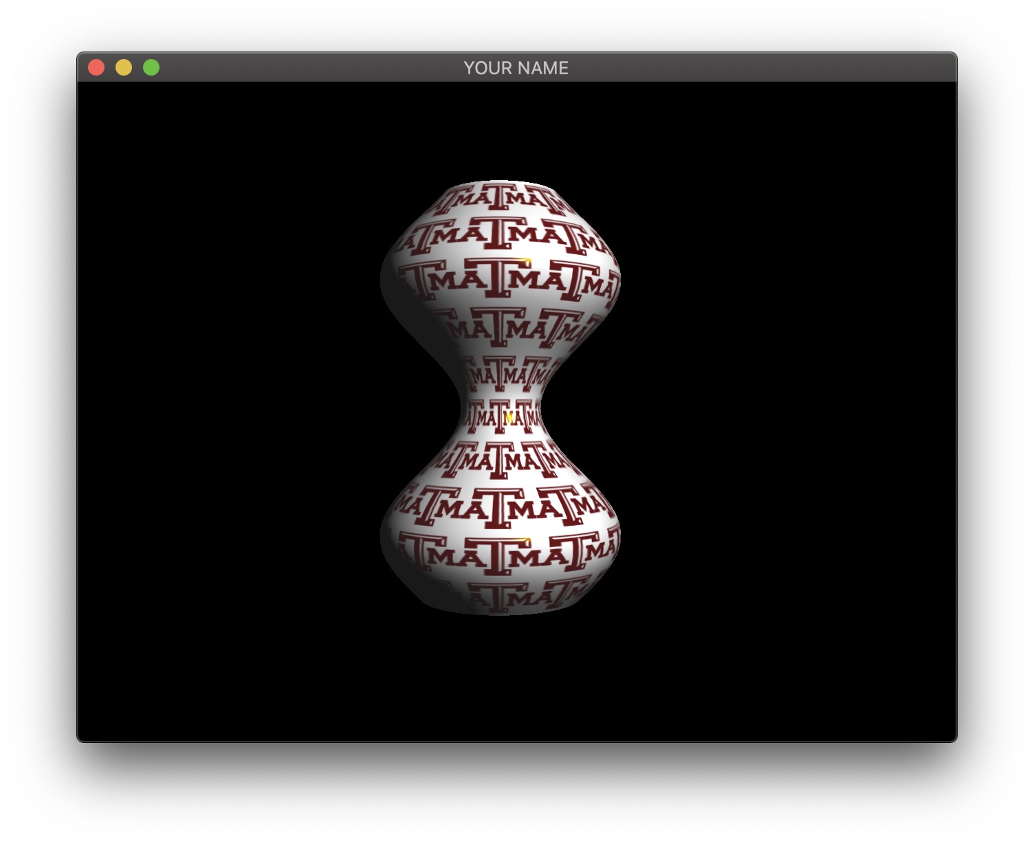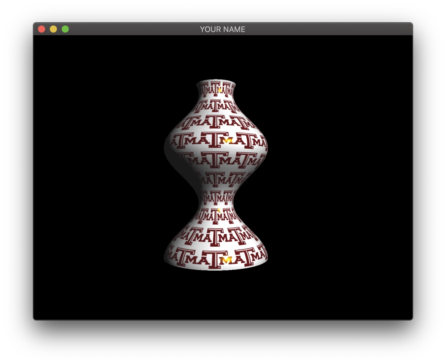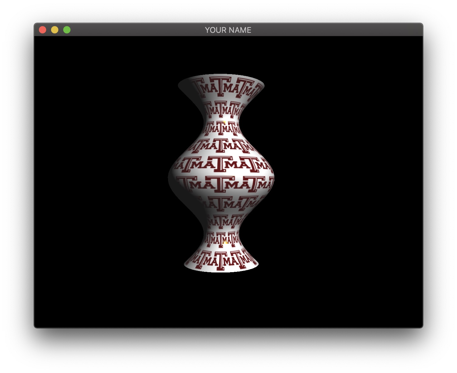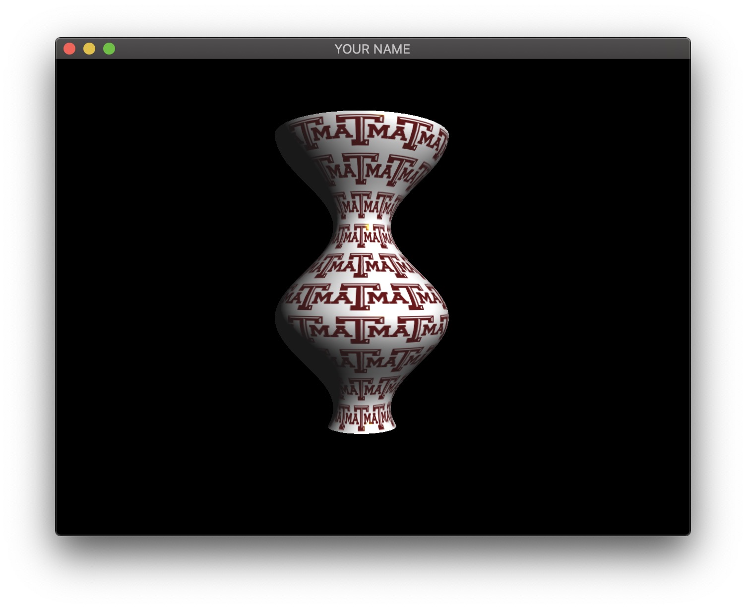
In this lab, we are going to create a vertex shader that computes a surface of revolution.

Start from your Lab 10 code. In this first task, we are going to create a surface of revolution on the CPU. We are going to create a scalar function \(y = f(x)\) and rotate this function around the X-axis. The function \(f(x)\) can be anything, but to avoid the surface from self-intersecting, the function should stay positive.
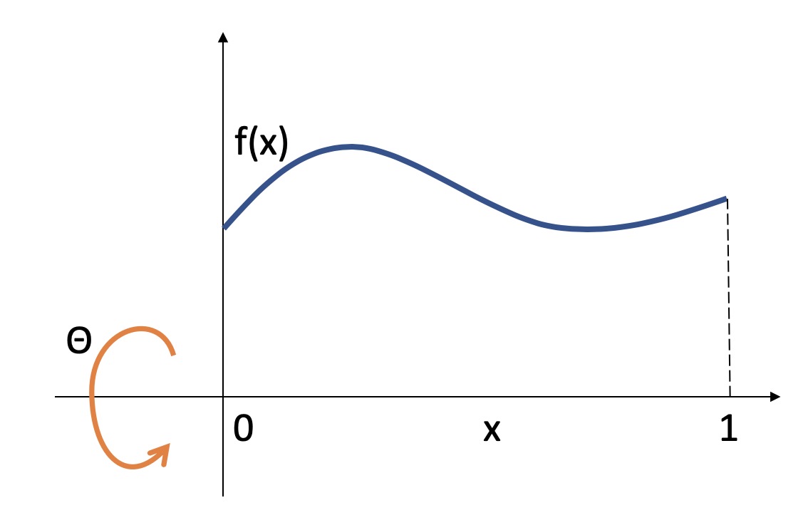
This means that we can parameterize a 3D surface point by \(x\) and \(\theta\): \[ \vec{p}(x, \theta) = \begin{pmatrix} x\\ f(x) \cos(\theta)\\ f(x) \sin(\theta) \end{pmatrix}. \]
For example, if you choose the function to be \(f(x) = \cos(x) + 2\), then the 3D position is: \[ \vec{p} = \begin{pmatrix} x\\ (\cos(x) + 2) \cos(\theta)\\ (\cos(x) + 2) \sin(\theta) \end{pmatrix}. \]
Note: for this particular choice of \(f(x)\), you may want to let \(x\) go from \(0\) to \(10\), rather than from \(0\) to \(1\). If you do this, you will need to apply a transform with the matrix stack to keep the overall scale reasonable. Alternatively, you can change the frequency of \(f(x)\) and let \(x\) go from \(0\) to \(1\).
You can create this surface using a double for-loop as in Lab \(10\):
for i = 1 ...
    for j = 1 ...
        x = ...
        theta = ...
        f = ...
        y = f * cos(theta)
        z = f * sin(theta)
    end
end
To compute the normal, you first need to compute the derivatives of \(\vec{p}\) with respect to \(x\) and \(\theta\): \[ \frac{d \vec{p}}{d x} = \begin{pmatrix} 1\\ f'(x) \cos(\theta)\\ f'(x) \sin(\theta) \end{pmatrix}, \quad \frac{d \vec{p}}{d \theta} = \begin{pmatrix} 0\\ -f(x) \sin(\theta)\\ f(x) \cos(\theta) \end{pmatrix}. \]
Using the example from before, \(f(x) = \cos(x) + 2\), the derivative is \(f'(x) = -\sin(x)\), so we get: \[ \frac{d \vec{p}}{d x} = \begin{pmatrix} 1\\ -\sin(x) \cos(\theta)\\ -\sin(x) \sin(\theta) \end{pmatrix}, \quad \frac{d \vec{p}}{d \theta} = \begin{pmatrix} 0\\ -(\cos(x) + 2) \sin(\theta)\\ (\cos(x) + 2) \cos(\theta) \end{pmatrix}. \]
Then take the cross product and normalize: \[ \vec{n} = \frac{d \vec{p}}{d x} \times \frac{d \vec{p}}{d \theta}, \quad \hat{n} = \frac{\vec{n}}{\|\vec{n}\|}. \]
To make this surface of revolution stand up along the Y axis, apply a rotation using the modelview matrix stack.
Now we’re going to move the computation to the GPU. In the C++ code, instead of sending \((x,y,z)\) in the position buffer, we are going to send \((x, \theta)\) and then evaluate the surface in the vertex shader.
To simplify the transition, we are going to keep the same buffer sizes for position, normal, and texture coordinates as before. In the double for-loop, remove (or comment out) the computation of the position and the normal, and instead send in just \(x\) and \(\theta\):
for i = 1 ...
    for j = 1 ...
        x = ...
        theta = ...
        // Position (send x and theta)
        posBuf.push_back(x);
        posBuf.push_back(theta);
        posBuf.push_back(0.0f);
        // Normal (send in zeros)
        norBuf.push_back(0.0f);
        norBuf.push_back(0.0f);
        norBuf.push_back(0.0f);
        // Texcoords (same as before)
        texBuf.push_back(...);
        texBuf.push_back(...);
    end
end
In the vertex shader, we have access to \(x\) and \(\theta\) through the position attribute variable. Using these, we can compute position \(\vec{p}\) and normal \(\hat{n}\). These quantities are in model space, so after these vectors are constructed, they need to be transformed to camera space using the modelview matrix (inverse transpose for the normal).
NOTE: Read the “Debugging OpenGL & GLSL” section in Assignment 2.
NOTE: The GLSL compiler will silently optimize away any variables that are not used in the shader. If you try to access these variables at runtime, the program will crash, since these variables no longer exist in the shader. In this lab, when you move the computation of the normal to the GPU, the aNor variable no longer needs to be passed to the GPU, since it is computed in the shader. Therefore, you will have to comment out any reference to aNor from your C++ runtime code. Or, you can trick the GLSL compiler from optimizing away aNor by using it and discarding it as follows:
vec3 nor = aNor.xyz;
nor.x = ...;
nor.y = ...;
nor.z = ...;Finally, we’re going to make the surface change with time. Pass in the current time as a uniform variable so that the function \(f(x)\) depends on time. In main.cpp’s render function, do something like this:
...
double t = glfwGetTime();
...
glUniform1f(prog->getUniform("t"), t);
...
And then in the vertex shader, do something like this:
...
uniform float t;
...
Now, make the function dependent on \(t\) as well: \(f(x,t)\). All of the equations from earlier still hold, except with the added time dependence. The normal computation will need to be updated to take \(t\). For example, we can turn our old function into \(f(x,t) = \cos(x + t) + 2\) and \(f'(x,t) = -\sin(x + t)\). Then we have: \[ \vec{p} = \begin{pmatrix} x\\ (\cos(x + t) + 2) \cos(\theta)\\ (\cos(x + t) + 2) \sin(\theta) \end{pmatrix}, \quad \frac{d \vec{p}}{d x} = \begin{pmatrix} 1\\ -\sin(x + t) \cos(\theta)\\ -\sin(x + t) \sin(\theta) \end{pmatrix}, \quad \frac{d \vec{p}}{d \theta} = \begin{pmatrix} 0\\ -(\cos(x + t) + 2) \sin(\theta)\\ (\cos(x + t) + 2) \cos(\theta) \end{pmatrix}. \]
