Assignments
Throughout the course you will be implementing various RL algorithms. Namely, Value Iteration, Asynchronous Value Iteration, Policy Iteration, Monte-Carlo Control, Monte-Carlo Control with Importance Sampling, Q-Learning, SARSA, Q-Learning with Approximation, Deep Q-Learning, REINFORCE, A2C, and DDPG. See below the implementation guidelines for each of the algorithms.
All your implementations will be within the provided codebase. You may work on your implementations at any time (even ahead of the lectures) as long as you submit your solutions on time.
By submitting assignments, students acknowledge and agree that their submissions will be sent to a non-secured third-party server for plagiarism detection. You should not to include any protected or private data in your submissions, as the processing of such data will occur on a non-secured server.
Instructions for setting up the assignment framework on your machine are provided here.
Tip: you might find it comfortable to use PyCharm for easy debugging. Follow this guide for setting and managing a virtual environment in PyCharm.
Executing
In order to execute the code, type python run.py along with the following arguments. If an argument is not provided, its default value is assumed.
- -s <solver> : Specify which RL algorithm to run. E.g., "-s vi" will exacute the Value Iteration algorithm. Default=random control.
- -d <domain> : Chosen environment from OpenAI Gym. E.g., "-d Gridworld" will run the Gridworld domain. Default="Gridworld".
- -o <name> : The result output file name. Default="out.csv".
- -e <int> : Number of episodes for training. Default=500.
- -t <int> : Maximal number of steps per episode. Default=10,000.
- -l <[int,int,...,int]> : Structure of a Deep neural net. E.g., "[10,15]" creates a net where the Input layer is connected to a hidden layer of size 10 that is connected to a hidden layer of size 15 that is connected to the output. Default=[24,24].
- -a <alpha> : The learning rate (alpha). Default=0.5.
- -r <seed> : Seed integer for a random stream. Default=random value from [0, 9999999999].
- -g <gamma> : The discount factor (gamma). Default=1.00.
- -p <epsilon> : Initial epsilon for epsilon greedy policies (can set up to decay over time). Default=0.1.
- -P <epsilon> : The minimum value of epsilon at which decaying is terminated (can be zero). Default=0.1.
- -c <rate> : Epsilon decay rate (can be 1 = no decay). Default=0.99.
- -m <size> : Size of the replay memory. Default=500,000.
- -N <n> : Copy parameters from the trained approximator to the target approximator every n steps. Default=10,000.
- -b <size> : Size of the training mini batches. Default=32.
- --no-plots; : Turn off the training curve online plotting.
Autograder
In order to run the autograder, type python autograder.py <solver> . For instance, to run autograder for Asynchronous Value Interation type python autograder.py avi . The autograder will print a total score out of 10, and will report failed test cases.
Note: The autograder is still in development, so make to sure to keep an eye on campuswire for updates to the file.
Help
Questions, comments, and clarifications regarding the assignments should NOT be sent via email to the course staff. Please use the class discussion board on Campuswire instead.
Submission
Each of the algorithms that you are required to implement has a separate '.py' file affiliated with it. When submitting an implementation, upload only the (single) '.py' file as a zip file named <your UIN>. For example, '123123123.zip'. Students auditing the class (not registered) are NOT allowed to upload a submission.
The 'ValueIteration' class in 'Value_Iteration.py' contains the implementation for the value iteration algorithm. Complete the 'train_episode' and 'create_greedy_policy' methods.
Resources
- Sutton & Barto, Section 4.4, page 82
Examples
- python run.py -s vi -d Gridworld -e 100 -g 0.9
- Converges in 3 episodes with reward of -26.24.
- python run.py -s vi -d Gridworld -e 100 -g 0.4
- Converges in 3 episodes with reward of -18.64.
- python run.py -s vi -d FrozenLake-v1 -e 100 -g 0.9
- Achieves a reward of 2.176 after 53 episodes.
The 'AsynchVI' class in 'Value_Iteration.py' contains an implementation for asynchronous value iteration. Complete the 'train_episode' method. You are expected to use prioritized sweeping to perform updates. An implementation of priority queque has been provided to you under 'Value_Iteration.py'.
Resources
- Sutton & Barto, Section 4.5, page 85
- 3MDPs.pptx, Slide 46
Examples
- python run.py -s avi -d FrozenLake-v1 -e 100 -g 0.5
- Reaches a reward of 0.637 after 50 episodes.
- python run.py -s avi -d FrozenLake-v1 -e 100 -g 0.7
- Reaches a reward of 0.978 after 88 episodes.
The 'PolicyIteration' class in 'Policy_Iteration.py' contains the implementation for the policy iteration algorithm. Complete the 'train_episode' and 'policy_eval' methods.
Resources
- Sutton & Barto, Section 4.3, page 80
- 3MDPs.pptx, Slides 52-53
Examples
- python run.py -s pi -d Gridworld -e 100 -g 0.9
- Converges in 4 episodes with reward of -26.24.
- python run.py -s pi -d Gridworld -e 100 -g 0.4
- Converges in 4 episodes with reward of -18.64.
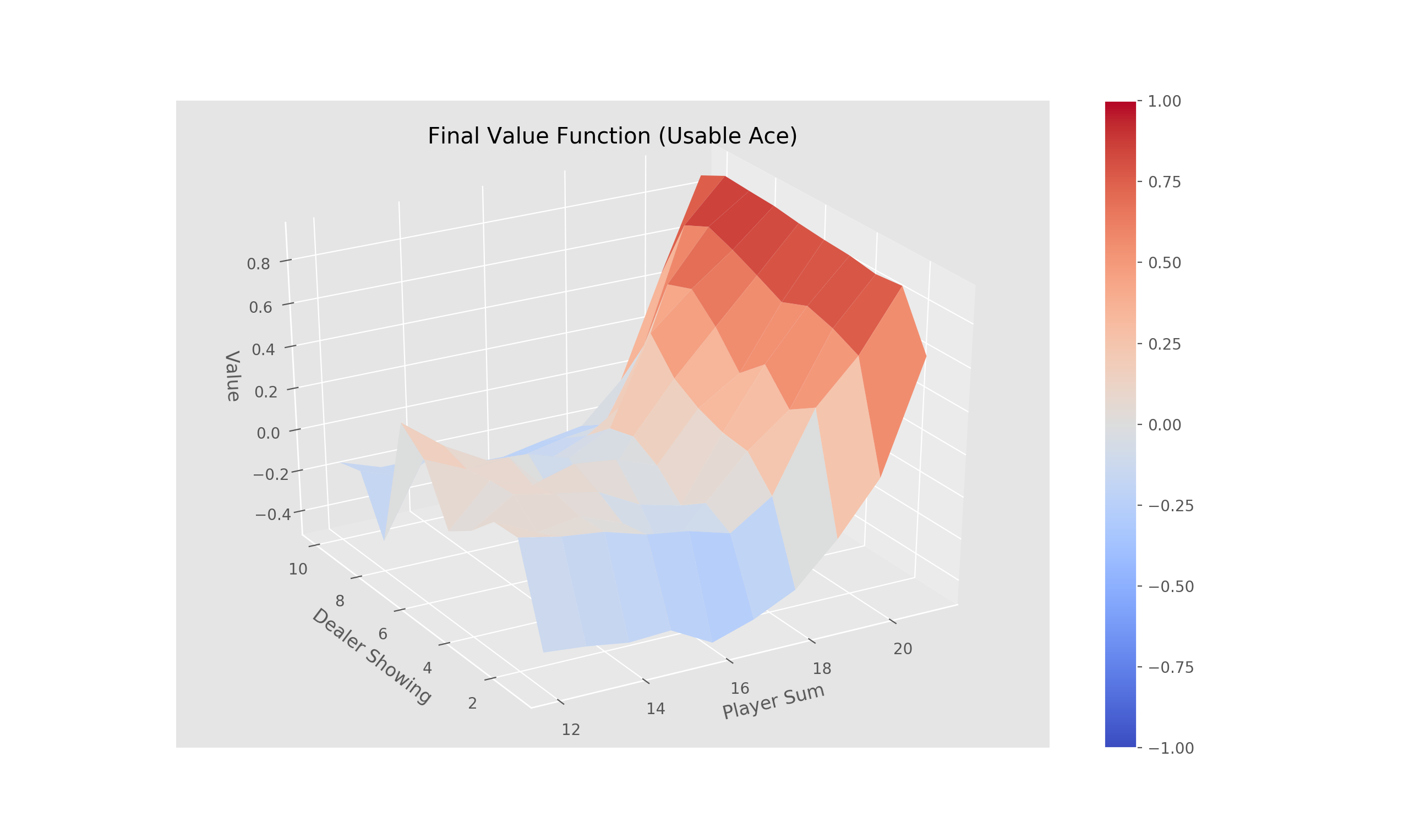
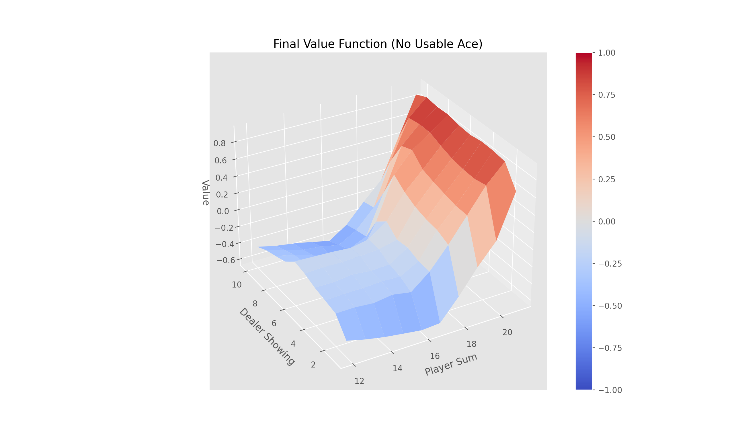
Complete the four methods, '__init__', 'train_episode', 'make_epsilon_greedy_policy', and 'create_greedy_policy', within the 'MonteCarlo' class in 'Monte_Carlo.py' that implements Monte-Carlo control using an epsilon-greedy policy. Recall that the parameter, '-p', sets the value of epsilon.
Resources
- Sutton & Barto, Section 5.4, page 100
Examples
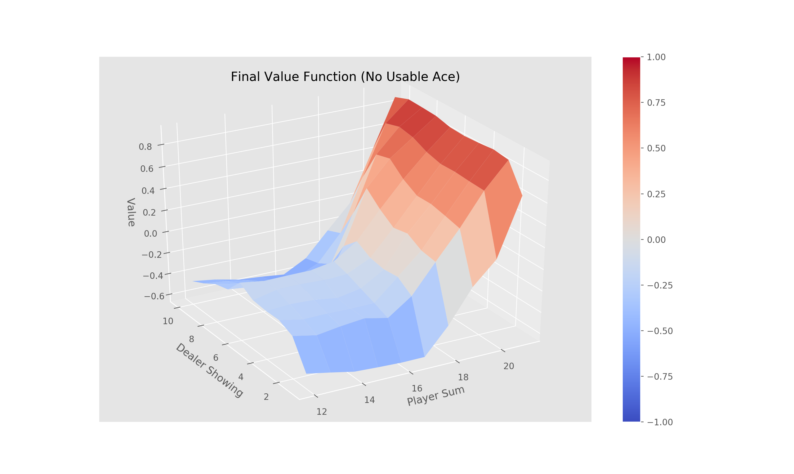
- python run.py -s mc -d Blackjack -e 500000 -g 1.0 -p 0.1
- python run.py -s mc -d Blackjack -e 500000 -g 0.8 -p 0.1

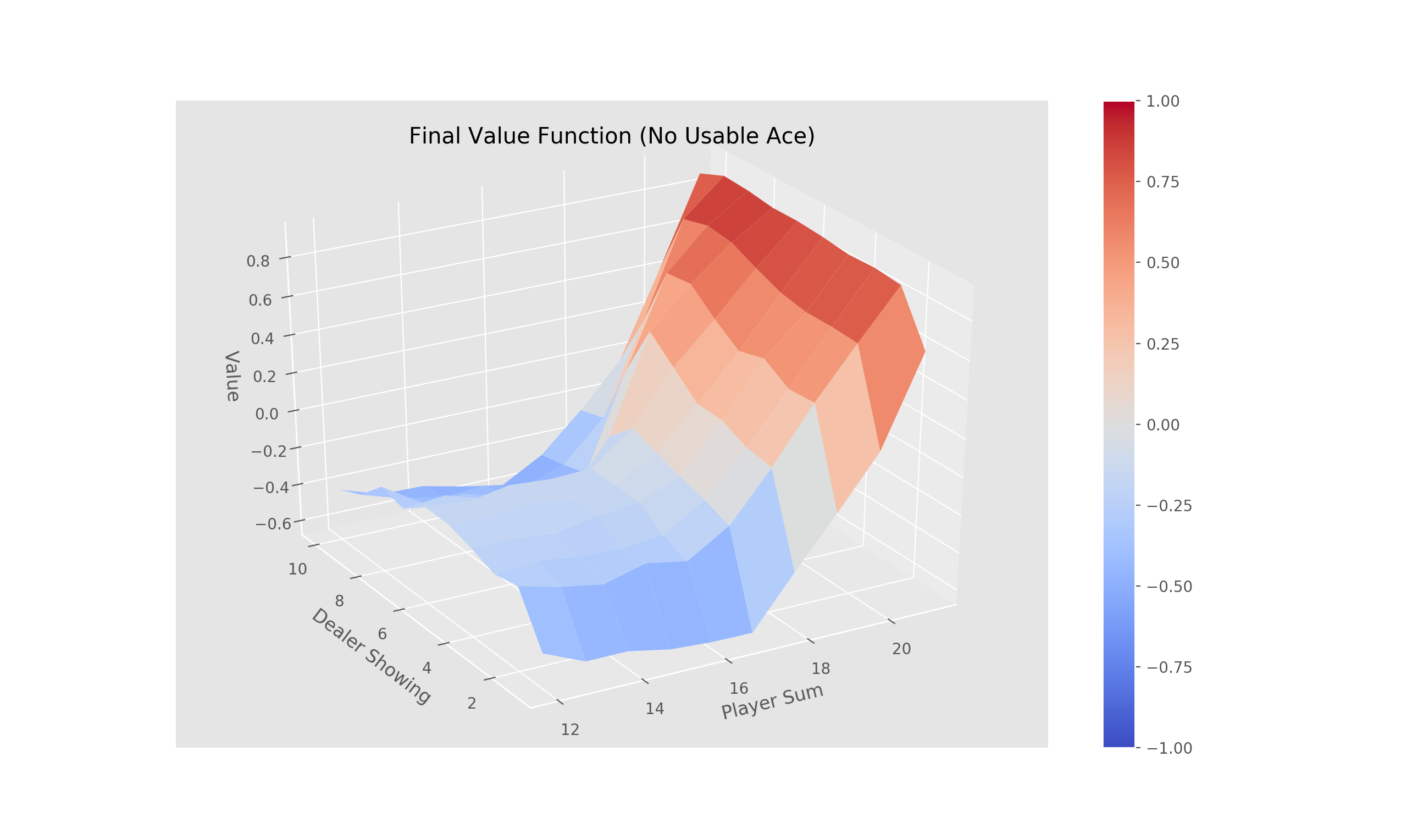
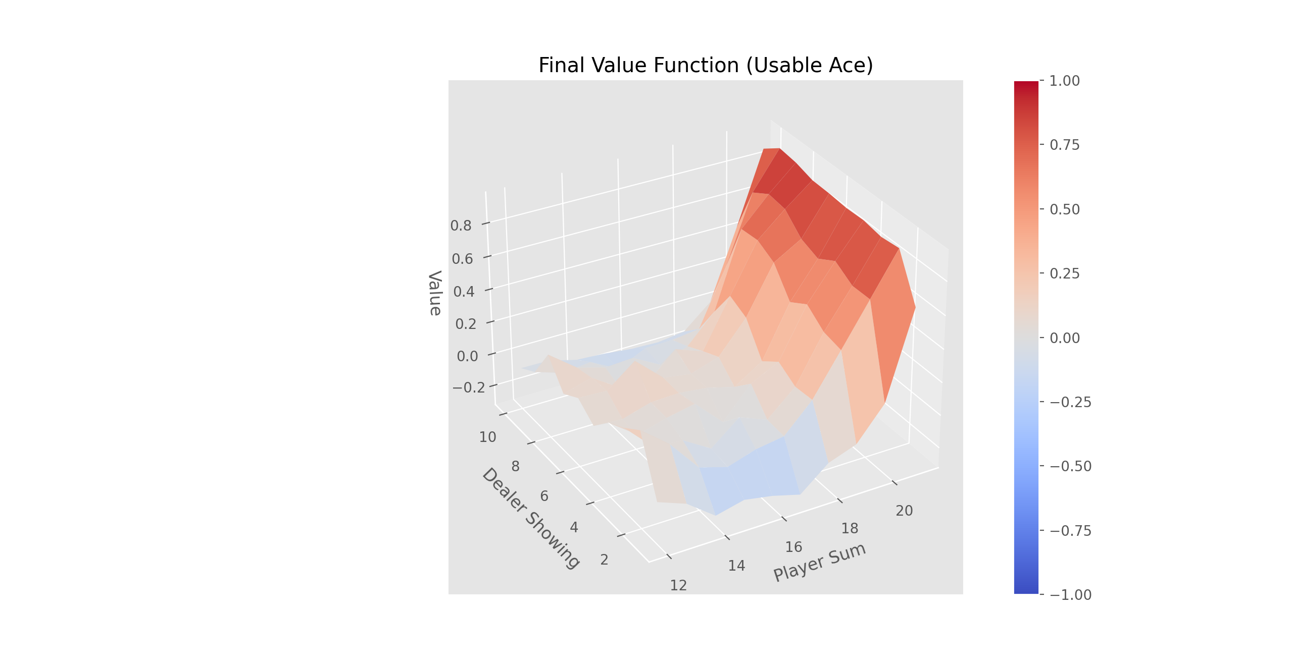
Complete the method 'train_episode' within the 'OffPolicyMC' class in 'Monte_Carlo.py' that implements off-policy Monte-Carlo control using weighted importance sampling. There is no need to define epsilon in this case as a random behavior policy is provided (for off-line learning).
Resources
- Sutton & Barto, Section 5.7, page 110
Examples
- python run.py -s mcis -d Blackjack -e 500000 -g 1.0
- python run.py -s mcis -d Blackjack -e 500000 -g 0.7


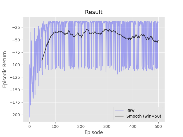
Complete the three methods, 'train_episode', 'create_greedy_policy', and 'make_epsilon_greedy_policy', within the 'QLearning' class in 'Q_Learning.py' that implements off-policy TD control (Q-Learning).
Resources
- Sutton & Barto, Section 6.5, page 131
Examples
- python run.py -s ql -d CliffWalking -e 500 -a 0.5 -g 1.0 -p 0.1
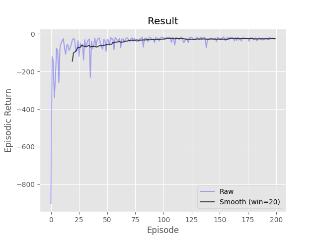
Complete the three methods, 'train_episode', 'create_greedy_policy', and 'make_epsilon_greedy_policy', within the 'Sarsa' class in 'Sarsa.py' that implements on-policy TD control (SARSA).
Resources
- Sutton & Barto, Section 6.4, page 129
Examples
- python run.py -s sarsa -d WindyGridworld -e 200 -a 0.5 -g 1.0 -p 0.1
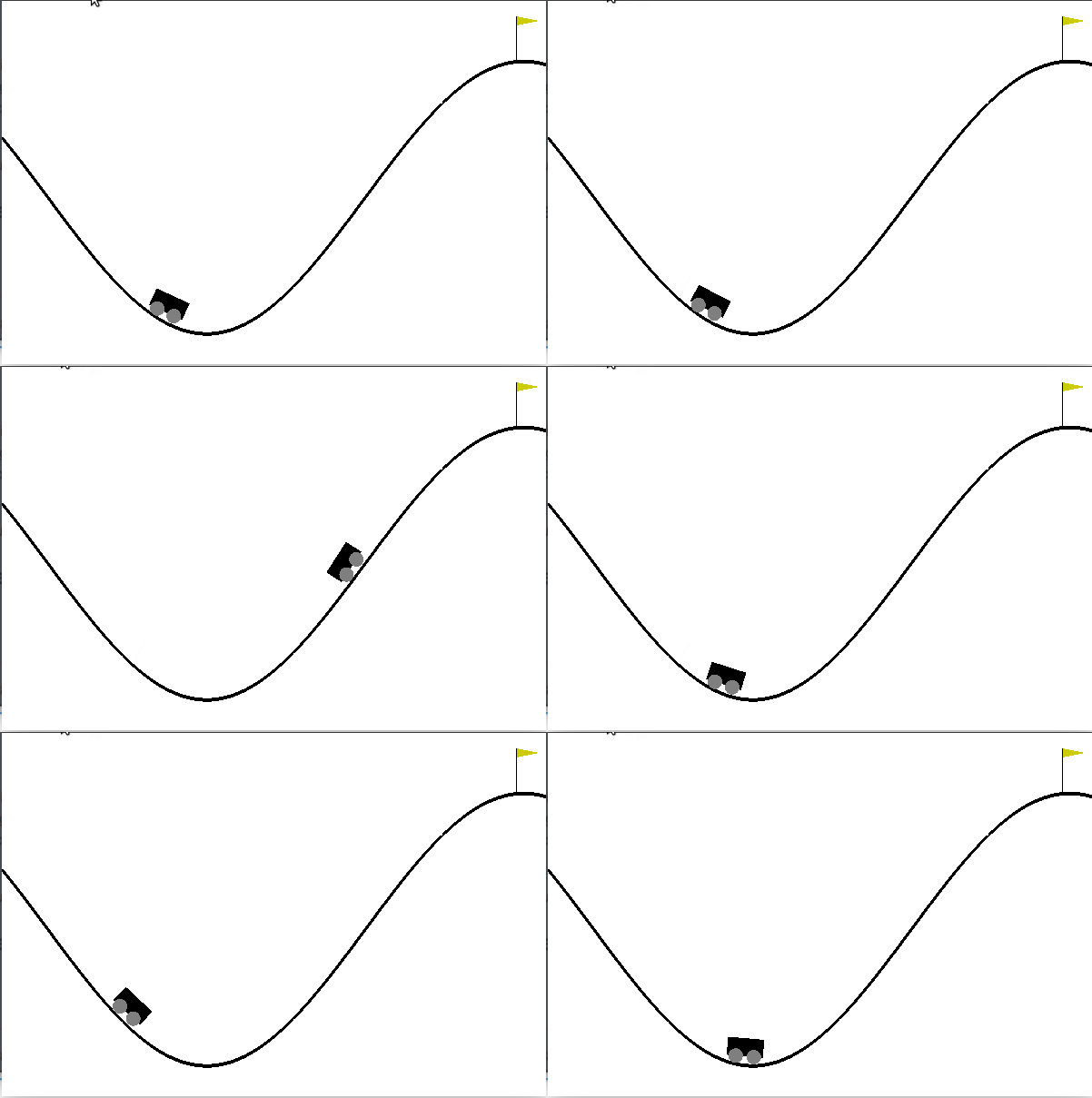
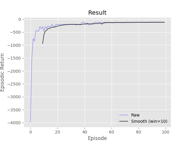
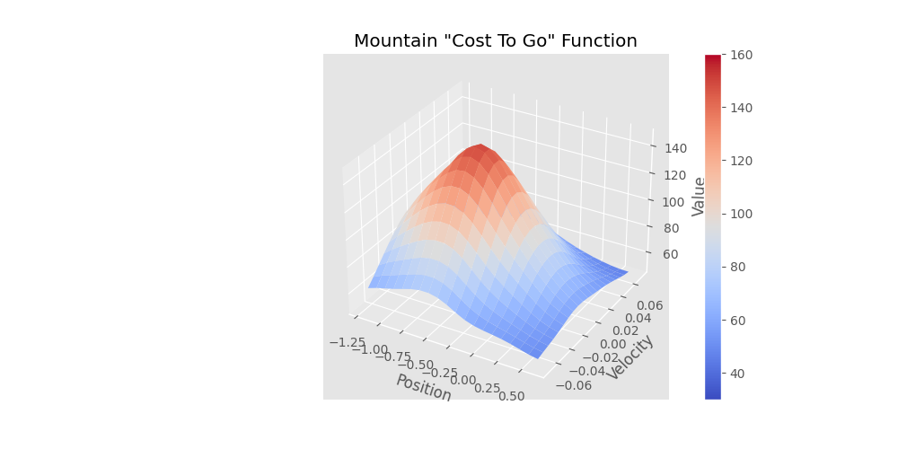
Complete the three methods, 'train_episode', 'create_greedy_policy', and 'make_epsilon_greedy_policy', within the 'ApproxQLearning' class in 'Q_Learning.py' that implements Q-Learning using a function approximator. A function approximator has been provided for you to use in the 'Estimator' class. The 'predict' function will return the estimated value of the given state and action. The 'update' function will adjust the weights of the approximator given the target value.
Resources
- Sutton & Barto, Section 6.5, page 131
- Sutton & Barto, Section 9.1, page 198
- Sutton & Barto, Chapter 11, page 257
Examples
- python run.py -s aql -d MountainCar-v0 -e 100 -g 1.0 -p 0.2
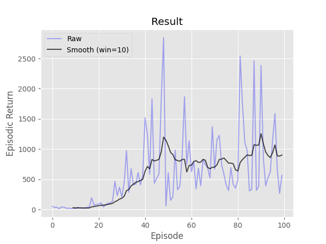
Complete the four methods, 'create_greedy_policy', 'epsilon_greedy', 'compute_target_values', and 'train_episode' within the 'DQN' class in 'DQN.py' implementing the DQN algorithm. A neural network has been initialized for you in the '__init__' function and a function, 'update_target_model', for copying it to the target network has been provided. You must create a memory of a size given by the parameter '-m' which is also known as a replay buffer. At each time step you should take an action given by the epsilon greedy policy (same as Q-learning), record the transition in memory, and update the online/active neural network. Apply a single update per time step with a minibatch of size '-b', selected uniformly from the memory. Refresh the target neural network at an interval equal to the parameter '-N'.
Resources
- Mnih et al. "Human-level control through deep reinforcement learning." nature 518.7540 (2015): 529-533
- Slide deck "12DQN.pptx"
Examples
- python run.py -s dqn -t 2000 -d CartPole-v1 -e 100 -a 0.01 -g 0.95 -p 1.0 -P 0.01 -c 0.95 -m 2000 -N 100 -b 32 -l [32,32]
- python run.py -s dqn -t 1000 -d LunarLander-v2 -e 500 -a 0.001 -g 0.99 -p 1.0 -P 0.05 -c 0.995 -m 10000 -N 100 -b 64 -l [128,128]


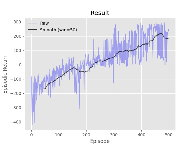
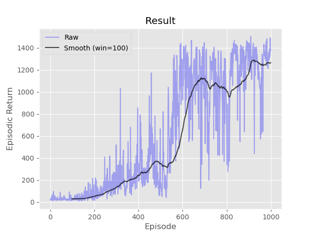
Complete the three methods, 'train_episode', 'compute_returns', and 'pg_loss', within the 'Reinforce' class in 'REINFORCE.py' implementing the 'REINFORCE' algorithm. A neural network has been initialized for you in the 'build_model' function. In 'train_episode', reset the environment, select an action by using the probabilities given by the neural network, and then at the conclusion of the episode update the network once using a batch containing all the transitions in the episode. In 'pg_loss' implement the loss function for policy gradient withouti> any additional improvements such as importance sampling or gradient clipping. Note that some improvements (normalization, Huber loss, etc.) have already been added to speed up learning. Keep in mind that policy gradient uses gradient ascent, but loss is minimized by auto-diff packages. Don't worry about matching the example too closely as multiple runs can have very different results using vanilla policy gradient.
Resources
- Sutton & Barto, Section 13.4, page 330
Examples
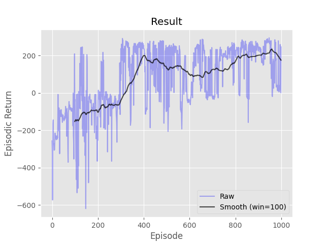
- python run.py -s reinforce -t 1000 -d CartPole-v1 -e 1000 -a 0.001 -g 0.99 -l [32,32]
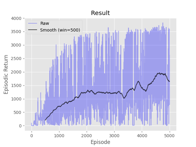
- python run.py -s reinforce -t 1000 -d LunarLander-v2 -e 5000 -a 0.0005 -g 0.99 -l [128,128]


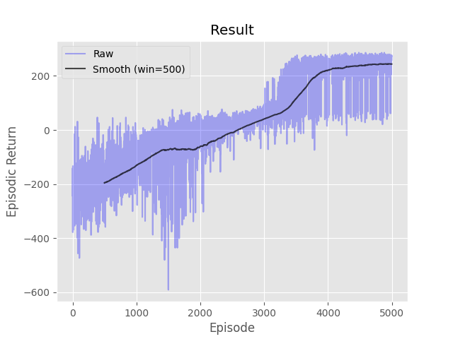
Complete the three methods, 'train_episode', 'actor_loss', and 'critic_loss' within the 'A2C' class in 'A2C.py' implementing the 'Advantage Actor Critic (A2C)' algorithm. Neural networks for the actor and the critic have been initialized for you in the '__init__' function. Keep in mind that the online actor-critic algorithm learns very slowly without using parallel workers due to the bias in the actor's updates (since the critic isn't perfect). Don't worry about matching the example too closely as multiple runs can have very different results using actor-critic methods without additional variance reduction tricks and/or hyperparameter tuning.
Resources
- Sutton & Barto, Section 13.5, page 332 (disregard the I variable)
- "14Actor-critic.pptx", slide 16.
Examples
- python run.py -s a2c -t 1000 -d CartPole-v1 -e 3000 -a 0.0001 -g 0.95 -l [64,64]
- python run.py -s a2c -t 1000 -d LunarLander-v2 -e 5000 -a 0.00005 -g 0.99 -l [128,128]

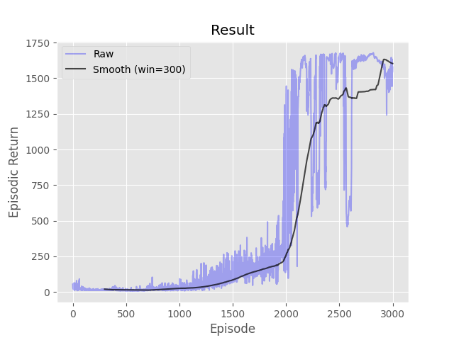

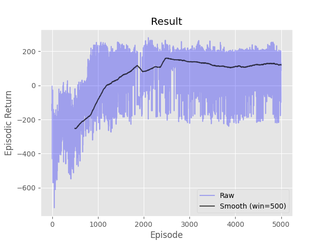
Complete the four methods, 'train_episode', 'compute_target_values', 'q_loss', and 'pi_loss' within the 'DDPG' class in 'DDPG.py' implementing the 'Deep Deterministic Policy Gradient (DDPG)' algorithm. Neural networks for the actor and the critic have been initialized for you in the '__init__' function. Don't worry about matching the example too closely as multiple runs can have very different results.
Resources
- OpenAI
- "16SAC.pptx", slide 27.
Examples
- python run.py -s ddpg -t 1000 -d LunarLanderContinuous-v2 -e 1000 -a 0.001 -g 0.99 -l [64,64] -b 100
- python run.py -s ddpg -t 1000 -d Hopper-v4 -e 5000 -a 0.001 -g 0.99 -l [256,256] -m 1000000 -b 100
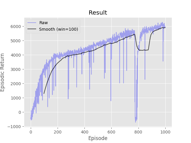
- python run.py -s ddpg -t 1000 -d HalfCheetah-v4 -e 1000 -a 0.001 -g 0.99 -l [256,256] -m 1000000 -b 100

