Assignments
The course's assignments apply an array of AI techniques to playing Pac-Man. However, these assignments don't focus on building AI for video games. Instead, they teach foundational AI concepts, such as informed state-space search, probabilistic inference, and reinforcement learning. These concepts underly real-world application areas such as natural language processing, computer vision, and robotics.
The assignments allow you to visualize the results of the techniques you implement. They also contain code examples and clear directions, but do not force you to wade through undue amounts of scaffolding. Finally, Pac-Man provides a challenging problem environment that demands creative solutions; real-world AI problems are challenging, and Pac-Man is too.
Technical Notes
The Pac-Man assignments are written in pure Python 3.6+ and do not depend on any packages external to a standard Python distribution, except the Logic and ML assignments.
Help
Questions, comments, and clarifications regarding the assignments should NOT be sent via email to the course staff. Please use the class discussion board on Canvas instead.
Submission
Each student is required to submit their own unique solution i.e., assignments should be completed alone. Assignments will by default be graded automatically for correctness, though we will review submissions individually as necessary to ensure that they receive the credit they deserve. Assignments can be submitted as often as you like before the deadline; we strongly encourage you to keep working until you get a full score by the autograder.
Credits
The assignments were developed by John DeNero, Dan Klein, and Pieter Abbeel at UC Berkeley.
This short tutorial introduces students to setup examples, the Python programming language, and the autograder system. Assignment 0 will cover the following:
- Instructions on how to set up Python,
- Workflow examples,
- A mini-Python tutorial,
- Assignment grading: Every assignment's release includes its autograder that you can run locally to debug. When you submit, the same autograder is ran.
Files to Edit and Submit: You will fill in
portions of addition.py,
buyLotsOfFruit.py,
and shopSmart.py
in tutorial.zip during the assignment. Once you have
completed the assignment, you will submit ONLY these files to Canvas zipped into a single
file.
Please DO NOT change/submit any other files.
Evaluation: Your code will be autograded for technical correctness. Please do not change the names of any provided functions or classes within the code, or you will wreak havoc on the autograder. However, the correctness of your implementation - not the autograder's judgements - will be the final judge of your score. If necessary, we will review and grade assignments individually to ensure that you receive due credit for your work.
Academic Dishonesty: We will be checking your code against other submissions in the class for logical redundancy. If you copy someone else's code and submit it with minor changes, we will know. These cheat detectors are quite hard to fool, so please don't try. We trust you all to submit your own work only; please don't let us down. If you do, we will pursue the strongest consequences available to us.
Python Installation
You need a Python (3.6 or higher) distribution and either Pip or Conda.
To check if you meet our requirements, you should open the terminal
run python -V
and see that the version is high enough. Then, run
pip -V and
conda -V
and see that at least one of these works and prints out some version
of the tool. On some systems that also have Python 2 you may have to
use python3
and pip3
instead of the aforementioned.
If you need to install things, we recommend Python 3.9 and Pip for simplicity. If you already have Python, you just need to install Pip.
On Windows either Windows Python or WSL2 can be used. WSL2 is really nice and provides a full Linux environment, but takes up more space; Linux/ MacOS (both Unix) is used much more often for computer science than Windows because it is more convenient and development tools are also more reliable. It doesn't make a difference for this class but is a good tool to learn to use if you are interested and have the time.
If you choose to use Conda via Anaconda or Miniconda, these already come with Python and Pip so you would install just the one thing.
- Install Python:
- For Windows and MacOS, we recommend using an official graphical installer: download and install Python 3.9.
- For Linux, use a package manager to install Python 3.9.
- Install Pip:
- For Windows and MacOS, run
python -m
                    ensurepip --upgrade
. - For Linux, use a package manager to install Pip for Python 3.
- For Windows and MacOS, run
Dependencies installation
First, go through the Autograding section to understand how to work
with tutorial.zip and the
autograder.py
inside.
The machine learning assignment has additional dependencies. It's important to install them now so that if there is an issue with the Python installation, we don't have to come back or redo the installation later.
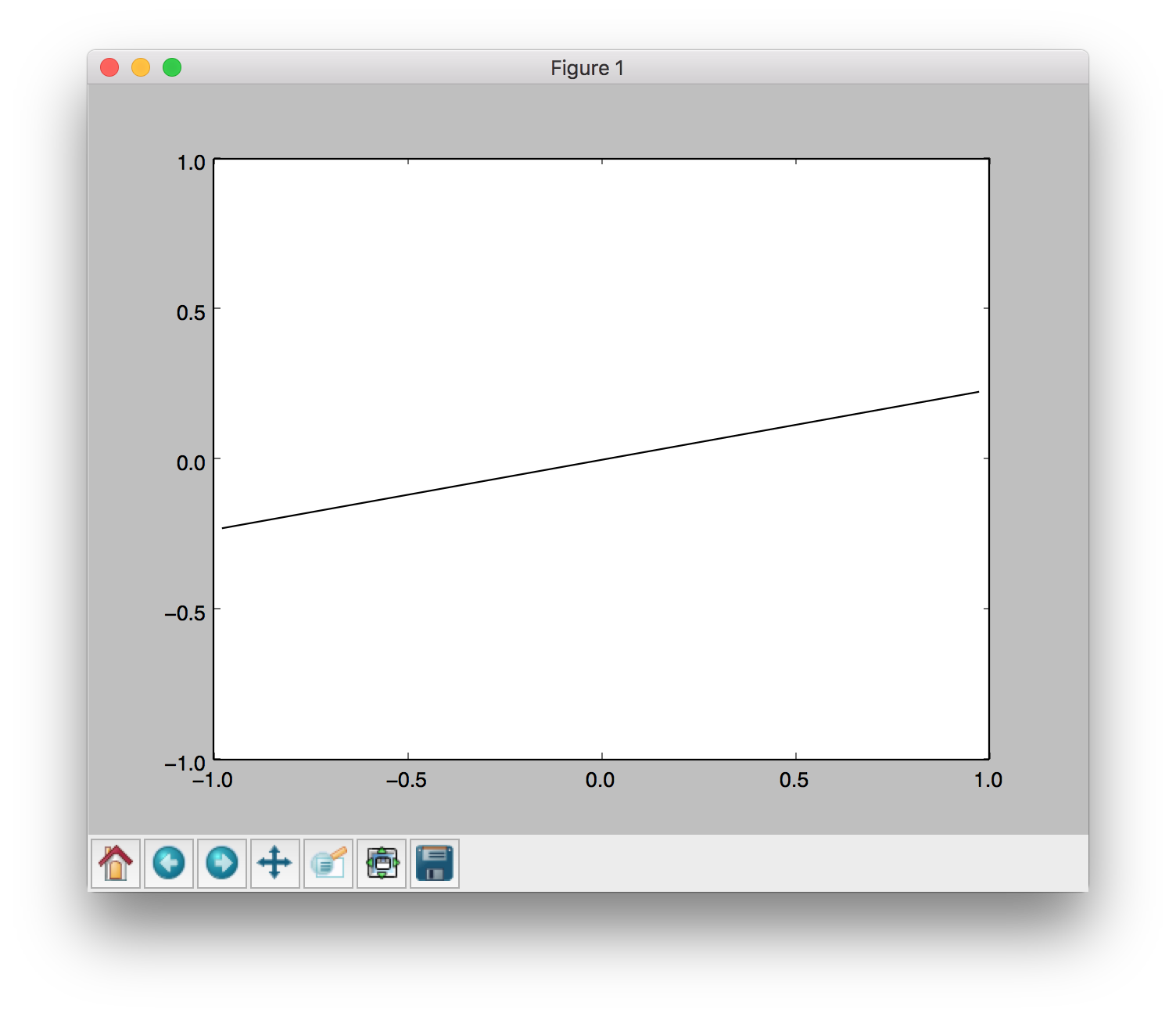
On Conda installations, the dependencies should already be there. You can test by confirming that this command produces the below window pop up where a line segment spins in a circle.
python autograder.py --check-dependencies
The libraries needed and the corresponding commands are:
- numpy, which provides support for fast, large multi-dimensional arrays.
- matplotlib, a 2D plotting library.
pip install numpy

pip install matplotlib
After these, use the python autograder.py --check-dependencies command to
confirm that everything works.
Troubleshooting
Some installations will have python3
and pip3
refer to what we want to use. Also, there may by multiple
installations of python that may complicate which commands install
where.
python -V # version of python
pip -V # version of pip, and which python it is installing to
          which python # where python is
If there is a tkinter
import error, it's likely because Python is atypical, and from
Homebrew. Uninstall that and install python from Homebrew with
tkinter
support, or use the recommended graphical installer.
Workflow/ Setup Examples
You are not expected to use a particular code editor or anything, but here are some suggestions on convenient workflows (you can skim both for half a minute and choose the one that looks better to you):
- GUI and IDE, with VS Code shortcuts. You are highly encouraged to read the Using an IDE section if using an IDE to learn convenient features.
- In terminal, using Unix commans and Emacs (this is fine to do on Windows too). Useful to be able to edit code on any machine without setup, and remote connecting setups such as using the instructional machines.
Python Basics
If you're new to Python or need a refresher, we recommend going through the Python basics tutorial.
Autograding
To get you familiarized with the autograder, we will ask you to code, test, and submit your code after solving the three questions.
You can download all of the files associated the autograder tutorial as a zip archive: tutorial.zip. Unzip this file and examine its contents:
          addition.py
          autograder.py
          buyLotsOfFruit.py
          grading.py
          projectParams.py
          shop.py
          shopSmart.py
          testClasses.py
          testParser.py
          test_cases
          tutorialTestClasses.py
This contains a number of files you'll edit or run:
addition.py: source file for question 1buyLotsOfFruit.py: source file for question 2shop.py: source file for question 3shopSmart.py: source file for question 3autograder.py: autograding script (see below)
and others you can ignore:
test_cases: directory contains the test cases for each questiongrading.py: autograder codetestClasses.py: autograder codetutorialTestClasses.py: test classes for this particular assignmentprojectParams.py: assignment parameters
The command python autograder.py grades your
solution to all three problems. If we run it before editing any files we get a page or two of output:
python autograder.py Should look as follows:
          [~/tutorial]$ python autograder.py
          Starting on 1-21 at 23:39:51

          Question q1
          ===========
          *** FAIL: test_cases/q1/addition1.test
          ***     add(a, b) must return the sum of a and b
          ***     student result: "0"
          ***     correct result: "2"
          *** FAIL: test_cases/q1/addition2.test
          ***     add(a, b) must return the sum of a and b
          ***     student result: "0"
          ***     correct result: "5"
          *** FAIL: test_cases/q1/addition3.test
          ***     add(a, b) must return the sum of a and b
          ***     student result: "0"
          ***     correct result: "7.9"
          *** Tests failed.

          ### Question q1: 0/1 ###


          Question q2
          ===========
          *** FAIL: test_cases/q2/food_price1.test
          ***     buyLotsOfFruit must compute the correct cost of the order
          ***     student result: "0.0"
          ***     correct result: "12.25"
          *** FAIL: test_cases/q2/food_price2.test
          ***     buyLotsOfFruit must compute the correct cost of the order
          ***     student result: "0.0"
          ***     correct result: "14.75"
          *** FAIL: test_cases/q2/food_price3.test
          ***     buyLotsOfFruit must compute the correct cost of the order
          ***     student result: "0.0"
          ***     correct result: "6.4375"
          *** Tests failed.

          ### Question q2: 0/1 ###


          Question q3
          ===========
          Welcome to shop1 fruit shop
          Welcome to shop2 fruit shop
          *** FAIL: test_cases/q3/select_shop1.test
          ***     shopSmart(order, shops) must select the cheapest shop
          ***     student result: "None"
          ***     correct result: "<FruitShop: shop1>"
          Welcome to shop1 fruit shop
          Welcome to shop2 fruit shop
          *** FAIL: test_cases/q3/select_shop2.test
          ***     shopSmart(order, shops) must select the cheapest shop
          ***     student result: "None"
          ***     correct result: "<FruitShop: shop2>"
          Welcome to shop1 fruit shop
          Welcome to shop2 fruit shop
          Welcome to shop3 fruit shop
          *** FAIL: test_cases/q3/select_shop3.test
          ***     shopSmart(order, shops) must select the cheapest shop
          ***     student result: "None"
          ***     correct result: "<FruitShop: shop3>"
          *** Tests failed.

          ### Question q3: 0/1 ###


          Finished at 23:39:51

          Provisional grades
          ==================
          Question q1: 0/1
          Question q2: 0/1
          Question q3: 0/1
          ------------------
          Total: 0/3

          Your grades are NOT yet registered.  To register your grades, make sure
          to follow your instructor's guidelines to receive credit on your assignment.
For each of the three questions, this shows the results of that question's tests, the questions grade, and a final summary at the end. Because you haven't yet solved the questions, all the tests fail. As you solve each question you may find some tests pass while other fail. When all tests pass for a question, you get full marks.
Looking at the results for question 1, you can see that it has failed three tests with the error message "add(a, b) must return the sum of a and b". The answer your code gives is always 0, but the correct answer is different. We'll fix that in the next tab.
Q1: Addition
Open addition.py
and look at the definition of add:
def add(a, b):
              "Return the sum of a and b"
              "*** YOUR CODE HERE ***"
              return 0
The tests called this with a and b set to different values, but the code always returned zero. Modify this definition to read:
def add(a, b):
              "Return the sum of a and b"
              print("Passed a = %s and b = %s, returning a + b = %s" % (a, b, a + b))
              return a + b
Now rerun the autograder (omitting the results for questions 2 and 3):
[~/tutorial]$ python autograder.py -q q1
          Starting on 1-22 at 23:12:08

          Question q1
          ===========

          *** PASS: test_cases/q1/addition1.test
          ***     add(a,b) returns the sum of a and b
          *** PASS: test_cases/q1/addition2.test
          ***     add(a,b) returns the sum of a and b
          *** PASS: test_cases/q1/addition3.test
          ***     add(a,b) returns the sum of a and b

          ### Question q1: 1/1 ###


          Finished at 23:12:08

          Provisional grades
          ==================
          Question q1: 1/1
          ------------------
          Total: 1/1
You now pass all tests, getting full marks for question 1. Notice
the new lines "Passed a=…" which appear before "*** PASS: …". These
are produced by the print statement in add.
You can use print statements like that to output information useful for debugging.
Q2: buyLotsOfFruit function
Implement the buyLotsOfFruit(orderList)
function in buyLotsOfFruit.py
which takes a list of (fruit,numPounds)
tuples and returns the cost of your list. If there is some
fruit in the list which doesn't appear in
fruitPrices it should print an error message and return
None.
Please do not change the fruitPrices
variable.
Run python autograder.py
until question 2 passes all tests and you get full marks. Each test
will confirm that
buyLotsOfFruit(orderList) returns the correct answer given
various possible inputs. For example,
test_cases/q2/food_price1.test tests whether:
Cost of
            [('apples', 2.0), ('pears', 3.0), ('limes', 4.0)] is 12.25
Q3: shopSmart function
Fill in the function shopSmart(orderList,fruitShops)
in shopSmart.py,
which takes an orderList (like the kind passed in to
FruitShop.getPriceOfOrder)
and a list of FruitShop
and returns the FruitShop
where your order costs the least amount in total. Don't change the
file name or variable names, please. Note that we will provide the
shop.py
implementation as a "support" file, so you don't need to submit yours.
Run python autograder.py
until question 3 passes all tests and you get full marks. Each test
will confirm that shopSmart(orderList,fruitShops)
returns the correct answer given various possible inputs. For
example, with the following variable definitions:
orders1 = [('apples', 1.0), ('oranges', 3.0)]
          orders2 = [('apples', 3.0)]
          dir1 = {'apples': 2.0, 'oranges': 1.0}
          shop1 =  shop.FruitShop('shop1',dir1)
          dir2 = {'apples': 1.0, 'oranges': 5.0}
          shop2 = shop.FruitShop('shop2', dir2)
          shops = [shop1, shop2]
test_cases/q3/select_shop1.test tests whether:
shopSmart.shopSmart(orders1, shops) == shop1
and test_cases/q3/select_shop2.test tests
whether: shopSmart.shopSmart(orders2, shops) == shop2
Submission
In order to submit your assignment, please upload the following files to
Canvas -> Assignments -> Assignment 0: addition.py,
buyLotsOfFruit.py,
and shopSmart.py. Upload the files in a single zip
file with your UIN as the file name i.e., <your UIN>.zip.
Students implement depth-first, breadth-first, uniform cost, and A* search algorithms. These algorithms are used to solve navigation and traveling salesman problems in the Pacman world.
In this assignment, your Pacman agent will find paths through his maze world, both to reach a particular location and to collect food efficiently. You will build general search algorithms and apply them to Pacman scenarios.
As in Assignment 0, this assignment includes an autograder for you to grade your answers on your machine. This can be run with the command:
python autograder.pySee the autograder tutorial in Assignment 0 for more information about using the autograder.
The code for this assignment consists of several Python files, some of which you will need to read and understand in order to complete the assignment, and some of which you can ignore. You can download all the code and supporting files as a search.zip.
Files you'll edit:
search.py: where all of your search algorithms will reside.searchAgents.py: where all of your search-based agents will reside.
Files you might want to look at:
pacman.py: the main file that runs Pacman games. This file describes a Pacman GameState type, which you use in this assignment.game.py: the logic behind how the Pacman world works. This file describes several supporting types like AgentState, Agent, Direction, and Grid.util.py: useful data structures for implementing search algorithms.
Supporting files you can ignore:
graphicsDisplay.py: graphics for PacmangraphicsUtils.py: support for Pacman graphicstextDisplay.py: ASCII graphics for PacmanghostAgents.py: agents to control ghostskeyboardAgents.py: keyboard interfaces to control Pacmanlayout.py: code for reading layout files and storing their contentsautograder.py: assignment autogradertestParser.py: parses autograder test and solution filestestClasses.py: general autograding test classestest_cases/: directory containing the test cases for each questionsearchTestClasses.py: assignment 1 specific autograding test classes
Files to Edit and Submit: You will fill in portions of search.py and searchAgents.py during the assignment. Once you have
completed the assignment, you will submit ONLY these files to Canvas zipped into a single
file.
Evaluation: Your code will be autograded for technical correctness. Please do not change the names of any provided functions or classes within the code, or you will wreak havoc on the autograder. However, the correctness of your implementation - not the autograder's judgements - will be the final judge of your score. If necessary, we will review and grade assignments individually to ensure that you receive due credit for your work.
Academic Dishonesty: We will be checking your code against other submissions in the class for logical redundancy. If you copy someone else's code and submit it with minor changes, we will know. These cheat detectors are quite hard to fool, so please don't try. We trust you all to submit your own work only; please don't let us down. If you do, we will pursue the strongest consequences available to us.
Getting Help: You are not alone! If you find yourself stuck on something, contact the course staff for help. Office hours and the course Campuswire are there for your support; please use them. We want these assignments to be rewarding and instructional, not frustrating and demoralizing.
Welcome to Pacman
After downloading the code, unzipping it, and changing to the directory, you should be able to play a game of Pacman by typing the following at the command line:
python pacman.pyPacman lives in a shiny blue world of twisting corridors and tasty round treats. Navigating this world efficiently will be Pacman's first step in mastering his domain.
The simplest agent in searchAgents.py is called
the GoWestAgent, which always goes West (a trivial
reflex agent). This agent can occasionally win:
python pacman.py --layout testMaze --pacman GoWestAgentBut, things get ugly for this agent when turning is required:
python pacman.py --layout tinyMaze --pacman GoWestAgentIf Pacman gets stuck, you can exit the game by typing CTRL-c into your terminal.
Soon, your agent will solve not only tinyMaze,
but any maze you want.
Note that pacman.py supports a number of options
that can each be expressed in a long way (e.g., --layout) or a short way (e.g., -l). You can see the list of all options and their
default values via:
python pacman.py -hAlso, all of the commands that appear in this assignment also appear in commands.txt, for easy copying and pasting. In
UNIX/Mac OS X, you can even run all these commands in order with bash commands.txt.
New Syntax
You may not have seen this syntax before:
def my_function(a: int, b: Tuple[int, int], c: List[List], d: Any, e: float=1.0):This is annotating the type of the arguments that Python should expect for this function. In the example
below, a should be an int -- integer, b should be a tuple of 2 ints, c should be a List of Lists of anything -- therefore a 2D array of anything,
d is essentially the same as not annotated and can
by anything, and e should be a float. e is also set to 1.0 if nothing is passed in for it,
i.e.:
my_function(1, (2, 3), [['a', 'b'], [None, my_class], [[]]], ('h', 1))The above call fits the type annotations, and doesn't pass anything in for e. Type annotations are meant to be an adddition to the docstrings to help you know what the functions are working with. Python itself doesn't enforce these. When writing your own functions, it is up to you if you want to annotate your types; they may be helpful to keep organized or not something you want to spend time on.
Q1 (3 pts): Finding a Fixed Food Dot using Depth First Search
In searchAgents.py, you'll find a fully
implemented SearchAgent, which plans out a path
through Pacman's world and then executes that path step-by-step. The search algorithms for formulating a
plan are not implemented -- that's your job.
First, test that the SearchAgent is working
correctly by running:
python pacman.py -l tinyMaze -p SearchAgent -a fn=tinyMazeSearchThe command above tells the SearchAgent to use
tinyMazeSearch as its search algorithm, which is
implemented in search.py. Pacman should navigate
the maze successfully.
Now it's time to write full-fledged generic search functions to help Pacman plan routes! Pseudocode for the search algorithms you'll write can be found in the lecture slides. Remember that a search node must contain not only a state but also the information necessary to reconstruct the path (plan) which gets to that state.
Important note: All of your search functions need to return a list of actions that will lead the agent from the start to the goal. These actions all have to be legal moves (valid directions, no moving through walls).
Important note: Make sure to use the Stack, Queue and PriorityQueue data structures provided to you in util.py! These data structure implementations have
particular properties which are required for compatibility with the autograder.
Hint: Each algorithm is very similar. Algorithms for DFS, BFS, UCS, and A* differ only in the details of how the fringe is managed. So, concentrate on getting DFS right and the rest should be relatively straightforward. Indeed, one possible implementation requires only a single generic search method which is configured with an algorithm-specific queuing strategy. (Your implementation need not be of this form to receive full credit).
Implement the depth-first search (DFS) algorithm in the depthFirstSearch function in search.py. To make your algorithm complete, write the
graph search version of DFS, which avoids expanding any already visited states.
Your code should quickly find a solution for:
python pacman.py -l tinyMaze -p SearchAgent
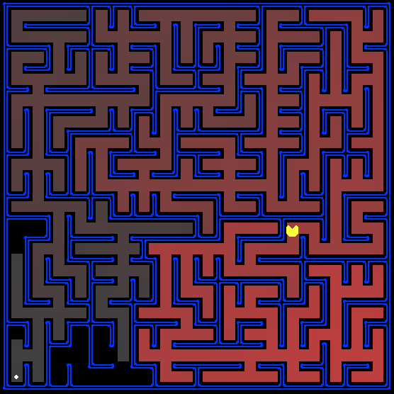
python pacman.py -l mediumMaze -p SearchAgent
python pacman.py -l bigMaze -z .5 -p SearchAgent
The Pacman board will show an overlay of the states explored, and the order in which they were explored (brighter red means earlier exploration). Is the exploration order what you would have expected? Does Pacman actually go to all the explored squares on his way to the goal?
Hint: If you use a Stack as your data structure,
the solution found by your DFS algorithm for mediumMaze should have a length of 130 (provided you
push successors onto the fringe in the order provided by getSuccessors; you might get 246 if you push them
in the reverse order). Is this a least cost solution? If not, think about what depth-first search is doing
wrong.
Grading: Please run the below command to see if your implementation passes all the autograder test cases.
python autograder.py -q q1
Q2 (3 pts): Breadth First Search
Implement the breadth-first search (BFS) algorithm in the breadthFirstSearch function in search.py. Again, write a graph search algorithm that
avoids expanding any already visited states. Test your code the same way you did for depth-first search.
python pacman.py -l mediumMaze -p SearchAgent -a fn=bfs
python pacman.py -l bigMaze -p SearchAgent -a fn=bfs -z .5
Does BFS find a least cost solution? If not, check your implementation.
Hint: If Pacman moves too slowly for you, try the option -- frameTime 0.
Note: If you've written your search code generically, your code should work equally well for the eight-puzzle search problem without any changes.
python eightpuzzle.py
Grading: Please run the below command to see if your implementation passes all the autograder test cases.
python autograder.py -q q2
Q3 (3 pts): Varying the Cost Function
While BFS will find a fewest-actions path to the goal, we might want to find paths that are "best" in other
senses. Consider mediumDottedMaze and mediumScaryMaze.
By changing the cost function, we can encourage Pacman to find different paths. For example, we can charge more for dangerous steps in ghost-ridden areas or less for steps in food-rich areas, and a rational Pacman agent should adjust its behavior in response.
Implement the uniform-cost graph search algorithm in the uniformCostSearch function in search.py. We encourage you to look through util.py for some data structures that may be useful in
your implementation. You should now observe successful behavior in all three of the following layouts, where
the agents below are all UCS agents that differ only in the cost function they use (the agents and cost
functions are written for you):
python pacman.py -l mediumMaze -p SearchAgent -a fn=ucs
python pacman.py -l mediumDottedMaze -p StayEastSearchAgent
python pacman.py -l mediumScaryMaze -p StayWestSearchAgent
Note: You should get very low and very high path costs for the StayEastSearchAgent and StayWestSearchAgent respectively, due to their
exponential cost functions (see searchAgents.py
for details).
Grading: Please run the below command to see if your implementation passes all the autograder test cases.
python autograder.py -q q3
Q4 (3 pts): A* search
Implement A* graph search in the empty function aStarSearch in search.py. A* takes a heuristic function as an
argument. Heuristics take two arguments: a state in the search problem (the main argument), and the problem
itself (for reference information). The nullHeuristic heuristic function in search.py is a trivial example.
You can test your A* implementation on the original problem of finding a path through a maze to a fixed
position using the Manhattan distance heuristic (implemented already as manhattanHeuristic in searchAgents.py).
python pacman.py -l bigMaze -z .5 -p SearchAgent -a fn=astar,heuristic=manhattanHeuristic
You should see that A* finds the optimal solution slightly faster than uniform cost search (about 549 vs.
620 search nodes expanded in our implementation, but ties in priority may make your numbers differ
slightly). What happens on openMaze for the
various search strategies?
Grading: Please run the below command to see if your implementation passes all the autograder test cases.
python autograder.py -q q4
Q5 (3 pts): Finding All the Corners
The real power of A* will only be apparent with a more challenging search problem. Now, it's time to formulate a new problem and design a heuristic for it.
In corner mazes, there are four dots, one in each corner. Our new search problem is to find the shortest
path through the maze that touches all four corners (whether the maze actually has food there or not). Note
that for some mazes like tinyCorners, the shortest
path does not always go to the closest food first! Hint: the shortest path through tinyCorners takes 28 steps.
Note: Make sure to complete Question 2 before working on Question 5, because Question 5 builds upon your answer for Question 2.
Implement the CornersProblem search problem in
searchAgents.py. You will need to choose a state
representation that encodes all the information necessary to detect whether all four corners have been
reached. Now, your search agent should solve:
python pacman.py -l tinyCorners -p SearchAgent -a fn=bfs,prob=CornersProblem
python pacman.py -l mediumCorners -p SearchAgent -a fn=bfs,prob=CornersProblem
To receive full credit, you need to define an abstract state representation that does not encode irrelevant
information (like the position of ghosts, where extra food is, etc.). In particular, do not use a Pacman
GameState as a search state. Your code will be
very, very slow if you do (and also wrong).
An instance of the CornersProblem class
represents an entire search problem, not a particular state. Particular states are returned by the functions
you write, and your functions return a data structure of your choosing (e.g. tuple, set, etc.) that
represents a state.
Furthermore, while a program is running, remember that many states simultaneously exist, all on the queue
of the search algorithm, and they should be independent of each other. In other words, you should not have
only one state for the entire CornersProblem
object; your class should be able to generate many different states to provide to the search algorithm.
Hint 1: The only parts of the game state you need to reference in your implementation are the starting Pacman position and the location of the four corners.
Hint 2: When coding up getSuccessors,
make sure to add children to your successors list with a cost of 1.
Our implementation of breadthFirstSearch expands
just under 2000 search nodes on mediumCorners.
However, heuristics (used with A* search) can reduce the amount of searching required.
Grading: Please run the below command to see if your implementation passes all the autograder test cases.
python autograder.py -q q5
Q6 (3 pts): Corners Problem: Heuristic
Note: Make sure to complete Question 4 before working on Question 6, because Question 6 builds upon your answer for Question 4.
Implement a non-trivial, consistent heuristic for the CornersProblem in cornersHeuristic.
python pacman.py -l mediumCorners -p AStarCornersAgent -z 0.5
Note: AStarCornersAgent is a shortcut for
-p SearchAgent -a fn=aStarSearch,prob=CornersProblem,heuristic=cornersHeuristic
Admissibility vs. Consistency: Remember, heuristics are just functions that take search states and return numbers that estimate the cost to a nearest goal. More effective heuristics will return values closer to the actual goal costs. To be admissible, the heuristic values must be lower bounds on the actual shortest path cost to the nearest goal (and non-negative). To be consistent, it must additionally hold that if an action has cost c, then taking that action can only cause a drop in heuristic of at most c.
Remember that admissibility isn't enough to guarantee correctness in graph search -- you need the stronger condition of consistency. However, admissible heuristics are usually also consistent, especially if they are derived from problem relaxations. Therefore it is usually easiest to start out by brainstorming admissible heuristics. Once you have an admissible heuristic that works well, you can check whether it is indeed consistent, too. The only way to guarantee consistency is with a proof. However, inconsistency can often be detected by verifying that for each node you expand, its successor nodes are equal or higher in in f-value. Moreover, if UCS and A* ever return paths of different lengths, your heuristic is inconsistent. This stuff is tricky!
Non-Trivial Heuristics: The trivial heuristics are the ones that return zero everywhere (UCS) and the heuristic which computes the true completion cost. The former won't save you any time, while the latter will timeout the autograder. You want a heuristic which reduces total compute time, though for this assignment the autograder will only check node counts (aside from enforcing a reasonable time limit).
Grading: Your heuristic must be a non-trivial non-negative consistent heuristic to receive any points. Make sure that your heuristic returns 0 at every goal state and never returns a negative value. Depending on how few nodes your heuristic expands, you'll be graded:
| Number of nodes expanded | Grade |
|---|---|
| more than 2000 | 0/3 |
| at most 2000 | 1/3 |
| at most 1600 | 2/3 |
| at most 1200 | 3/3 |
Remember: If your heuristic is inconsistent, you will receive no credit, so be careful!
Grading: Please run the below command to see if your implementation passes all the autograder test cases.
python autograder.py -q q6
Q7 (4 pts): Eating All The Dots
Now we'll solve a hard search problem: eating all the Pacman food in as few steps as possible. For this,
we'll need a new search problem definition which formalizes the food-clearing problem: FoodSearchProblem in searchAgents.py (implemented for you). A solution is
defined to be a path that collects all of the food in the Pacman world. For the present assignment,
solutions
do not take into account any ghosts or power pellets; solutions only depend on the placement of walls,
regular food and Pacman. (Of course ghosts can ruin the execution of a solution! We'll get to that in the
next assignment.) If you have written your general search methods correctly, A* with a null heuristic
(equivalent to uniform-cost search) should quickly find an optimal solution to testSearch with no code change on your part (total
cost of 7).
python pacman.py -l testSearch -p AStarFoodSearchAgent
Note: AStarFoodSearchAgent is a shortcut for
-p SearchAgent -a fn=astar,prob=FoodSearchProblem,heuristic=foodHeuristic
You should find that UCS starts to slow down even for the seemingly simple tinySearch. As a reference, our implementation takes
2.5 seconds to find a path of length 27 after expanding 5057 search nodes.
Note: Make sure to complete Question 4 before working on Question 7, because Question 7 builds upon your answer for Question 4.
Fill in foodHeuristic in searchAgents.py with a consistent heuristic
for the FoodSearchProblem. Try your agent on the
trickySearch board:
python pacman.py -l trickySearch -p AStarFoodSearchAgent
Our UCS agent finds the optimal solution in about 13 seconds, exploring over 16,000 nodes.
Any non-trivial non-negative consistent heuristic will receive 1 point. Make sure that your heuristic returns 0 at every goal state and never returns a negative value. Depending on how few nodes your heuristic expands, you'll get additional points:
| Number of nodes expanded | Grade |
|---|---|
| more than 15000 | 1/4 |
| at most 15000 | 2/4 |
| at most 12000 | 3/4 |
| at most 9000 | 4/4 (full credit; medium) |
| at most 7000 | 5/4 (optional extra credit; hard) |
Remember: If your heuristic is inconsistent, you will receive no credit, so be careful! Can you solve mediumSearch in a short time? If so, we're either
very, very impressed, or your heuristic is inconsistent.
Grading: Please run the below command to see if your implementation passes all the autograder test cases.
python autograder.py -q q7
Q8 (3 pts): Suboptimal Search
Sometimes, even with A* and a good heuristic, finding the optimal path through all the dots is hard. In
these cases, we'd still like to find a reasonably good path, quickly. In this section, you'll write an agent
that always greedily eats the closest dot. ClosestDotSearchAgent is implemented for you in searchAgents.py, but it's missing a key function that
finds a path to the closest dot.
Implement the function findPathToClosestDot in
searchAgents.py. Our agent solves this maze
(suboptimally!) in under a second with a path cost of 350:
python pacman.py -l bigSearch -p ClosestDotSearchAgent -z .5
Hint: The quickest way to complete findPathToClosestDot is to fill in the AnyFoodSearchProblem, which is missing its goal test.
Then, solve that problem with an appropriate search function. The solution should be very short!
Your ClosestDotSearchAgent won't always find the
shortest possible path through the maze. Make sure you understand why and try to come up with a small
example where repeatedly going to the closest dot does not result in finding the shortest path for eating
all the dots.
Grading: Please run the below command to see if your implementation passes all the autograder test cases.
python autograder.py -q q8
Submission
In order to submit your assignment, please upload the following files to
Canvas -> Assignments -> Assignment 1: Search search.py and
searchAgents.py. Upload the files in a single zip
file with your UIN as the file name i.e., <your UIN>.zip.
Students will apply the search algorithms and problems implemented in A1 to handle more difficult scenarios that include controlling multiple pacman agents and planning under time constraints.
Overview
In this contest, you will apply the search algorithms and problems implemented in Assignment 1 to handle more difficult scenarios that include controlling multiple pacman agents and planning under time constraints. There is room to bring your own unique ideas, and there is no single set solution. Much looking forward to seeing what you come up with!
Grading
Grading is assigned according to the following key:
- +1 points per staff bot (3 in total) beaten in the final ranking
- +0.1 points per student bot beaten in the final ranking
- 1st place: +2 points
- 2nd and 3rd place: +1.5 points
Quick Start Guide
- Download all the code and supporting files
contest1.zip, unzip it, and change to the directory. - Copy your
search.pyfrom Assignment 1 into the minicontest1 directory (replacing the blanksearch.py). - Go into
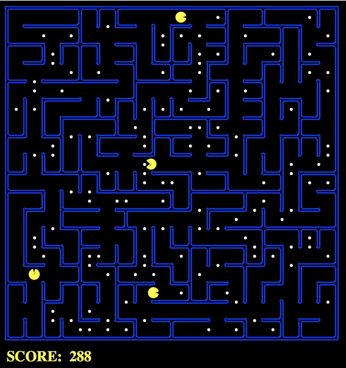
myAgents.pyand fill outfindPathToClosestDotinClosestDotAgent, andisGoalStateinAnyFoodSearchProblem. You should be able to copy your solutions from Assignment 1 over. - Run
and you should be able to see 4 pacman agents travelling around the map collecting dots.
python pacman.py - Submit the
myAgents.pyfile to Contest 1 on Canvas.
Important! You only need to submit myAgents.py. If you import from search.py
or searchProblems.py, the autograder will use
the staff version of those files.
Introduction
The base code is nearly identical to Assignment 1, but with some minor modifications to include support for more than one Pacman agent. You can download all the code and supporting files as a zip archive. Some key differences:
- You will control
NPacman agents on the board at a time. Your code must be able to support a multiple number of agents. - There is a cost associate with how long Pacman "thinks" (compute cost). See Scoring for more details.
Files you'll edit:
myAgents.py: What will be submitted. Contains all of the code needed for your agent.
Files you might want to look at:
searchProblems.py: The same code as in A1, with some slight modifications.search.py: The same code as in A1.pacman.py: The main file that runs Pacman games. This file describes a Pacman GameState type, which you use in this contest.
Files to Edit and Submit: You will fill and submit myAgents.py
Evaluation: Your code will be autograded for technical correctness. Please do not change the names of any provided functions or classes within the code, or you will wreak havoc on the autograder. However, the correctness of your implementation -- not the autograder's judgements -- will be the final judge of your score. If necessary, we will review and grade assignments individually to ensure that you receive due credit for your work.
Academic Dishonesty: We will be checking your code against other submissions in the class for logical redundancy. If you copy someone else's code and submit it with minor changes, we will know. These cheat detectors are quite hard to fool, so please don't try. We trust you all to submit your own work only; please don't let us down. If you do, we will pursue the strongest consequences available to us.
Getting Help: You are not alone! If you find yourself stuck on something, contact the course staff for help. Office hours and the course Campuswire are there for your support; please use them. We want these assignments to be rewarding and instructional, not frustrating and demoralizing.
Discussion: Please be careful not to post spoilers.
Rules
Layout
There are a variety of layout in the layouts
directory. Agents will be exposed to a variety
of maps of different sizes and amounts of food.
Scoring
The scoring from Assignment 1 is maintained, with a few modifications
Kept from Assignment 1
- +10 for each food pellet eaten
- +500 for collecting all food pellets
Modifications
- -0.4 for each action taken (Assignment 1 penalized -1)
- -1 *
total compute used to calculate next action (in seconds)* 1000
Each agent also starts with 100 points.
Observations
Each agent can see the entire state of the game, such as
food pellet locations, all pacman locations, etc. See the GameState
section for more details.
Winning and Losing
Win: You win if you collect all food pellets. Your score is the current amount of points.
Lose: You lose if your score reaches zero. This can be caused by not finding pellets quickly enough, or spending too much time on compute. Your score for this game is zero. If your agent crashes, it automatically receives a score of zero.
Designing Agents
File Format
You should include your agents in a file of the same format as myAgents.py. Your agents must
be completely contained in this one file. Though, you may use the functions in
search.py.
Interface
The GameState in pacman.py should look familiar, but contains some
modifications to support multiple Pacman agents. The major change to note is that many GameState methods
now have an extra argument, agentIndex, which is
to identify which Pacman agent it needs. For
example, state.getPacmanPosition(0) will get the
position of the first pacman agent. For more
information,
see the GameState class inpacman.py.
Agent
To get started designing your own agent, we recommend subclassing the
Agent class in game.py
(this has already been done by default). This provides to one important variable, self.index,
which is the agentIndex of the current agent.
For example, if we have 2 agents, each agent
will be created with a unique index, [MyAgent(index=0), MyAgent(index=1)], that can be
used
when deciding on actions.
The autograder will call the createAgents
function to create your team of pacman. By
default, it is set to create N identical pacmen,
but you may modify the code to return a
diverse team of multiple types of agents
Getting Started
By default, the game runs with the ClosestDotAgent implemented in the Quick Start Guide. To run your own agent, change agent for
the createAgents
method in myAgents.py
python pacman.pyA wealth of options are available to you:
python pacman.py --helpTo run a game with your agent, do:
python pacman.py --pacman myAgents.pyLayouts
The layouts folder contains all of the test
cases that will be executed on the autograder. To see how you perform on
any single map, you can run
python pacman.py --layout test1.layTesting
You can run you agent on a single test by using the following command. See the layouts
folder for the full suite of tests. There are no hidden tests
python pacman.py --layout test1.layYou can run the autograder by running the command below. Your score may vary from the autograder due to differences between machines, as well as staff vs student search implementations.
python autograder.py --pacman myAgents.pyClassic Pacman is modeled as both an adversarial and a stochastic search problem. Students implement multiagent minimax and expectimax algorithms, as well as designing evaluation functions.
In this assignment, you will design agents for the classic version of Pacman, including ghosts. Along the way, you will implement both minimax and expectimax search and try your hand at evaluation function design.
The code base has not changed much from the previous assignment, but please start with a fresh installation, rather than intermingling files from assignment 1.
As in assignment 1, this assignment includes an autograder for you to grade your answers on your machine. This can be run on all questions with the command:
python autograder.py
It can be run for one particular question, such as q2, by:
python autograder.py -q q2
It can be run for one particular test by commands of the form:
python autograder.py -t test_cases/q2/0-small-tree
By default, the autograder displays graphics with the -t option, but doesn't with the -q option. You can force graphics by using the --graphics flag, or force no graphics by using the
--no-graphics flag.
See the autograder tutorial in Assignment 0 for more information about using the autograder.
The code for this assignment contains the following files, available as a zip archive.
| Files you'll edit: | |
multiAgents.py |
Where all of your multi-agent search agents will reside. |
| Files you might want to look at: | |
pacman.py |
The main file that runs Pacman games. This file also describes a Pacman GameState type, which you will use extensively in this assignment. |
game.py |
The logic behind how the Pacman world works. This file describes several supporting types like AgentState, Agent, Direction, and Grid. |
util.py |
Useful data structures for implementing search algorithms. You don't need to use these for this assignment, but may find other functions defined here to be useful. |
| Supporting files you can ignore: | |
graphicsDisplay.py |
Graphics for Pacman |
graphicsUtils.py |
Support for Pacman graphics |
textDisplay.py |
ASCII graphics for Pacman |
ghostAgents.py |
Agents to control ghosts |
keyboardAgents.py |
Keyboard interfaces to control Pacman |
layout.py |
Code for reading layout files and storing their contents |
autograder.py |
Assignment autograder |
testParser.py |
Parses autograder test and solution files |
testClasses.py |
General autograding test classes |
test_cases/ |
Directory containing the test cases for each question |
multiagentTestClasses.py |
Assignment 2 specific autograding test classes |
Files to Edit and Submit: You will fill in portions of multiAgents.py during the assignment. Once you have
completed the assignment, you will submit ONLY these files to Canvas zipped into a single
file.
Evaluation: Your code will be autograded for technical correctness. Please do not change the names of any provided functions or classes within the code, or you will wreak havoc on the autograder. However, the correctness of your implementation -- not the autograder's judgements -- will be the final judge of your score. If necessary, we will review and grade assignments individually to ensure that you receive due credit for your work.
Academic Dishonesty: We will be checking your code against other submissions in the class for logical redundancy. If you copy someone else's code and submit it with minor changes, we will know. These cheat detectors are quite hard to fool, so please don't try. We trust you all to submit your own work only; please don't let us down. If you do, we will pursue the strongest consequences available to us.
Getting Help: You are not alone! If you find yourself stuck on something, contact the course staff for help. Office hours and the course Campuswire are there for your support; please use them. We want these assignments to be rewarding and instructional, not frustrating and demoralizing.
Discussion: Please be careful not to post spoilers.
Welcome to Multi-Agent Pacman
First, play a game of classic Pacman by running the following command:
python pacman.py
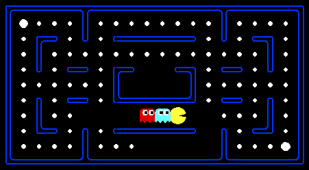
and using the arrow keys to move. Now, run the provided ReflexAgent in multiAgents.py
python pacman.py -p ReflexAgent
Note that it plays quite poorly even on simple layouts:
python pacman.py -p ReflexAgent -l testClassic
Inspect its code (in multiAgents.py) and make
sure
you understand what it's doing.
Q1 (4 pts): Reflex Agent
Improve the ReflexAgent in multiAgents.py to play respectably. The provided
reflex
agent code provides some helpful examples of methods that query the GameState for information. A capable reflex agent will
have to consider both food locations and ghost locations to perform well. Your agent should easily and
reliably clear the testClassic layout:
python pacman.py -p ReflexAgent -l testClassic
Try out your reflex agent on the default mediumClassic layout with one ghost or two (and
animation off to speed up the display):
python pacman.py --frameTime 0 -p ReflexAgent -k 1
python pacman.py --frameTime 0 -p ReflexAgent -k 2
How does your agent fare? It will likely often die with 2 ghosts on the default board, unless your evaluation function is quite good.
Note: Remember that newFood has the
function asList()
Note: As features, try the reciprocal of important values (such as distance to food) rather than just the values themselves.
Note: The evaluation function you're writing is evaluating state-action pairs; in later parts of the assignment, you'll be evaluating states.
Note: You may find it useful to view the internal contents of various objects for debugging. You
can
do this by printing the objects' string representations. For example, you can print newGhostStates with print(newGhostStates).
Options: Default ghosts are random; you can also play for fun with slightly smarter directional ghosts
using
-g DirectionalGhost. If the randomness is
preventing
you from telling whether your agent is improving, you can use -f to run with a fixed random seed (same random
choices
every game). You can also play multiple games in a row with -n. Turn off graphics with -q to run lots of games quickly.
Grading: We will run your agent on the openClassic layout 10 times. You will receive 0 points
if your agent times out, or never wins. You will receive 1 point if your agent wins at least 5 times, or 2
points if your agent wins all 10 games. You will receive an additional 1 point if your agent's average score
is greater than 500, or 2 points if it is greater than 1000. You can try your agent out under these
conditions
with
python autograder.py -q q1
To run it without graphics, use:
python autograder.py -q q1 --no-graphics
Don't spend too much time on this question, though, as the meat of the assignment lies ahead.
Q2 (5 pts): Minimax
Now you will write an adversarial search agent in the provided MinimaxAgent class stub in multiAgents.py. Your minimax agent should work with
any
number of ghosts, so you'll have to write an algorithm that is slightly more general than what you've
previously seen in lecture. In particular, your minimax tree will have multiple min layers (one for each
ghost) for every max layer.
Your code should also expand the game tree to an arbitrary depth. Score the leaves of your minimax tree
with
the supplied self.evaluationFunction, which
defaults
to scoreEvaluationFunction. MinimaxAgent extends MultiAgentSearchAgent, which gives access to self.depth and self.evaluationFunction. Make sure your minimax code
makes reference to these two variables where appropriate as these variables are populated in response to
command line options.
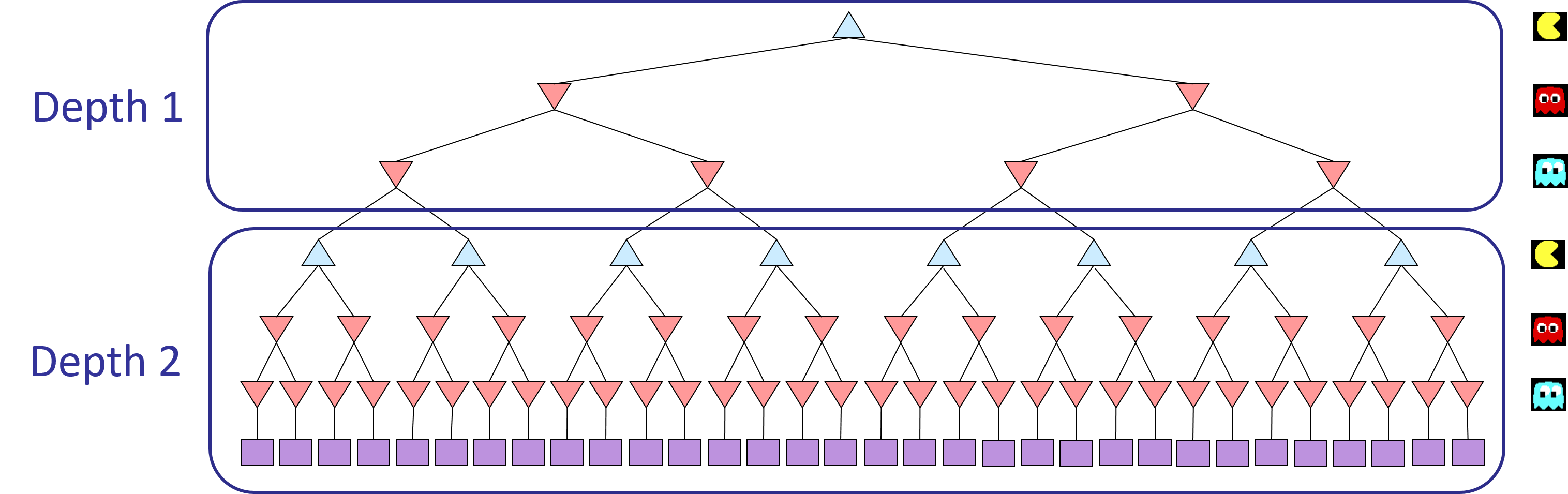
Important: A single search ply is considered to be one Pacman move and all the ghosts' responses, so depth 2 search will involve Pacman and each ghost moving two times (see diagram below).
Grading: We will be checking your code to determine whether it explores the correct number of game
states. This is the only reliable way to detect some very subtle bugs in implementations of minimax. As a
result, the autograder will be very picky about how many times you call GameState.generateSuccessor. If you call it any more
or
less than necessary, the autograder will complain. To test and debug your code, run
python autograder.py -q q2
This will show what your algorithm does on a number of small trees, as well as a pacman game. To run it without graphics, use:
python autograder.py -q q2 --no-graphics
Hints and Observations
- Implement the algorithm recursively using helper function(s).
- The correct implementation of minimax will lead to Pacman losing the game in some tests. This is not a problem: as it is correct behaviour, it will pass the tests.
- The evaluation function for the Pacman test in this part is already written (
self.evaluationFunction). You shouldn't change this function, but recognize that now we're evaluating states rather than actions, as we were for the reflex agent. Look-ahead agents evaluate future states whereas reflex agents evaluate actions from the current state. - The minimax values of the initial state in the
minimaxClassiclayout are 9, 8, 7, -492 for depths 1, 2, 3 and 4 respectively. Note that your minimax agent will often win (665/1000 games for us) despite the dire prediction of depth 4 minimax.python pacman.py -p MinimaxAgent -l minimaxClassic -a depth=4 - Pacman is always agent 0, and the agents move in order of increasing agent index.
- All states in minimax should be
GameStates, either passed in togetActionor generated viaGameState.generateSuccessor. In this assignment, you will not be abstracting to simplified states. - On larger boards such as
openClassicandmediumClassic(the default), you'll find Pacman to be good at not dying, but quite bad at winning. He'll often thrash around without making progress. He might even thrash around right next to a dot without eating it because he doesn't know where he'd go after eating that dot. Don't worry if you see this behavior, question 5 will clean up all of these issues. - When Pacman believes that his death is unavoidable, he will try to end the game as soon as possible
because of the constant penalty for living. Sometimes, this is the wrong thing to do with random ghosts,
but
minimax agents always assume the worst:
python pacman.py -p MinimaxAgent -l trappedClassic -a depth=3Make sure you understand why Pacman rushes the closest ghost in this case.
Q3 (5 pts): Alpha-Beta Pruning
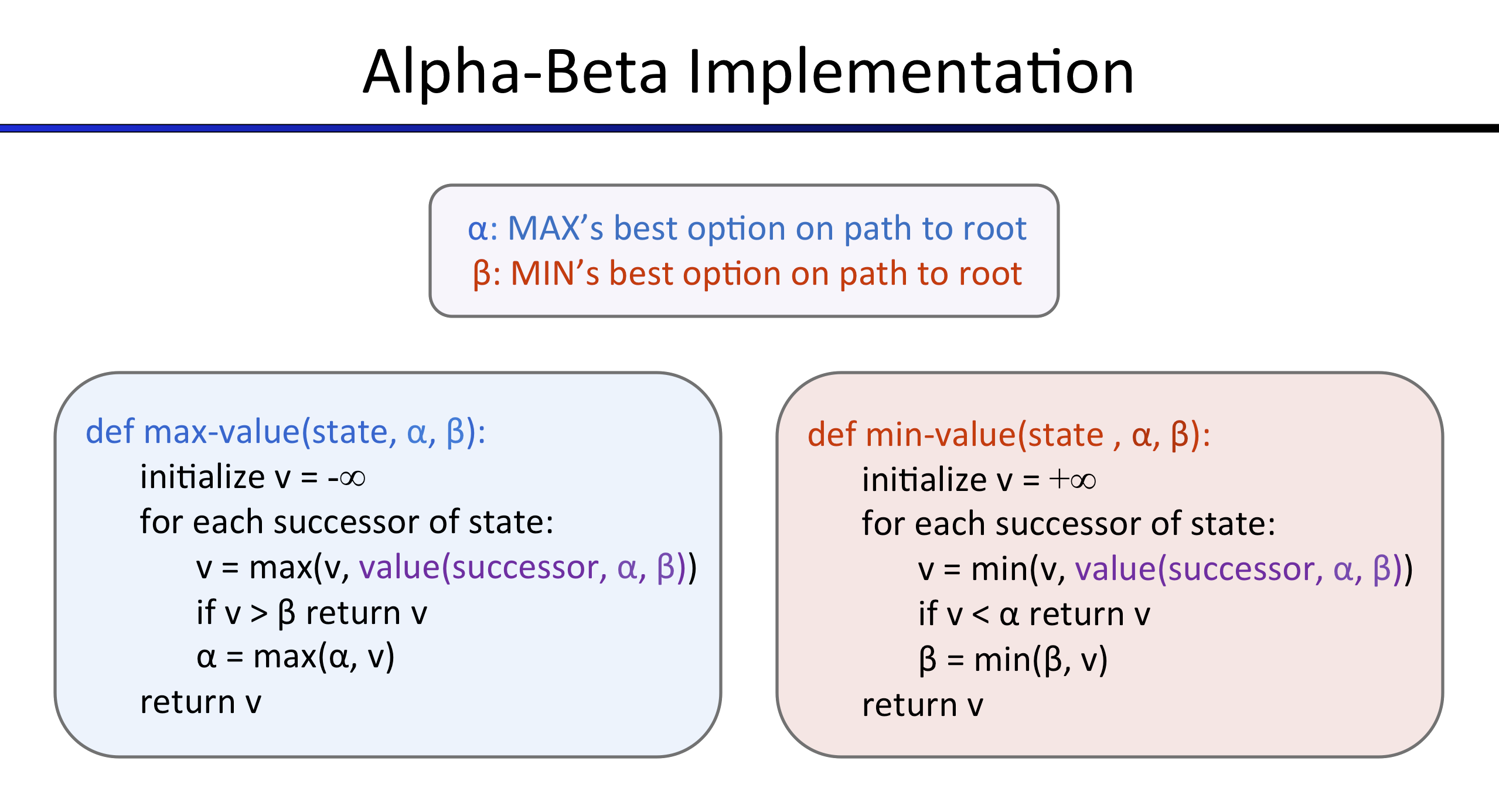
Make a new agent that uses alpha-beta pruning to more efficiently explore the minimax tree, in AlphaBetaAgent. Again, your algorithm will be slightly
more general than the pseudocode from lecture, so part of the challenge is to extend the alpha-beta pruning
logic appropriately to multiple minimizer agents.
You should see a speed-up (perhaps depth 3 alpha-beta will run as fast as depth 2 minimax). Ideally, depth
3
on smallClassic should run in just a few seconds
per
move or faster.
python pacman.py -p AlphaBetaAgent -a depth=3 -l smallClassic
The AlphaBetaAgent minimax values should be
identical to the MinimaxAgent minimax values,
although the actions it selects can vary because of different tie-breaking behavior. Again, the minimax
values
of the initial state in the minimaxClassic layout
are 9, 8, 7 and -492 for depths 1, 2, 3 and 4 respectively.
Grading: Because we check your code to determine whether it explores the correct number of states,
it is important that you perform alpha-beta pruning without reordering children. In other words, successor
states should always be processed in the order returned by GameState.getLegalActions. Again, do not call GameState.generateSuccessor more than necessary.
You must not prune on equality in order to match the set of states explored by our autograder. (Indeed, alternatively, but incompatible with our autograder, would be to also allow for pruning on equality and invoke alpha-beta once on each child of the root node, but this will not match the autograder.)
The pseudo-code below represents the algorithm you should implement for this question.
To test and debug your code, run
python autograder.py -q q3
This will show what your algorithm does on a number of small trees, as well as a pacman game. To run it without graphics, use:
python autograder.py -q q3 --no-graphics
The correct implementation of alpha-beta pruning will lead to Pacman losing some of the tests. This is not a problem: as it is correct behaviour, it will pass the tests.
Q4 (5 pts): Expectimax
Minimax and alpha-beta are great, but they both assume that you are playing against an adversary who makes
optimal decisions. As anyone who has ever won tic-tac-toe can tell you, this is not always the case. In this
question you will implement the ExpectimaxAgent,
which is useful for modeling probabilistic behavior of agents who may make suboptimal choices.
As with the search and problems yet to be covered in this class, the beauty of these algorithms is their general applicability. To expedite your own development, we've supplied some test cases based on generic trees. You can debug your implementation on small the game trees using the command:
python autograder.py -q q4
Debugging on these small and manageable test cases is recommended and will help you to find bugs quickly.
Once your algorithm is working on small trees, you can observe its success in Pacman. Random ghosts are of
course not optimal minimax agents, and so modeling them with minimax search may not be appropriate. ExpectimaxAgent will no longer take the min over all
ghost actions, but the expectation according to your agent's model of how the ghosts act. To simplify your
code, assume you will only be running against an adversary which chooses amongst their getLegalActions uniformly at random.
To see how the ExpectimaxAgent behaves in Pacman, run:
python pacman.py -p ExpectimaxAgent -l minimaxClassic -a depth=3
You should now observe a more cavalier approach in close quarters with ghosts. In particular, if Pacman perceives that he could be trapped but might escape to grab a few more pieces of food, he'll at least try. Investigate the results of these two scenarios:
python pacman.py -p AlphaBetaAgent -l trappedClassic -a depth=3 -q -n 10
python pacman.py -p ExpectimaxAgent -l trappedClassic -a depth=3 -q -n 10
You should find that your ExpectimaxAgent wins
about half the time, while your AlphaBetaAgent
always loses. Make sure you understand why the behavior here differs from the minimax case.
The correct implementation of expectimax will lead to Pacman losing some of the tests. This is not a problem: as it is correct behaviour, it will pass the tests.
Q5 (6 pts): Evaluation Function
Write a better evaluation function for Pacman in the provided function betterEvaluationFunction. The evaluation function
should
evaluate states, rather than actions like your reflex agent evaluation function did. With depth 2 search,
your
evaluation function should clear the smallClassic
layout with one random ghost more than half the time and still run at a reasonable rate (to get full credit,
Pacman should be averaging around 1000 points when he's winning).
Grading: the autograder will run your agent on the smallClassic layout 10 times. We will assign points to your evaluation function in the following way:
- If you win at least once without timing out the autograder, you receive 1 points. Any agent not satisfying these criteria will receive 0 points.
- +1 for winning at least 5 times, +2 for winning all 10 times
- +1 for an average score of at least 500, +2 for an average score of at least 1000 (including scores on lost games)
- +1 if your games take on average less than 30 seconds on the autograder machine, when run with
--no-graphics. - The additional points for average score and computation time will only be awarded if you win at least 5 times.
You can try your agent out under these conditions with
python autograder.py -q q5
To run it without graphics, use:
python autograder.py -q q5 --no-graphics
Students will implement an agent for playing the repeated prisoner dilemma game.

Overview
In this contest, you will implement an agent for playing the
repeated prisoner dilemma game. This game has a twist in the form
of uncertainty regarding the reported opponent action from the
previous round. The contest code is available as a zip
archive (contest2.zip).
There is room to bring your own unique ideas, and there is no single set solution. We look forward to seeing what you come up with!
Quick Start Guide
- Download the code (
contest2.zip), unzip it, and change to the directory. - Go into
Players/MyPlayer.pyand fill out your UINs separated by ‘:' (not by ‘,') in the "UIN" field, choose a team name at "your team name", Write your strategy under the "play" function. Your strategy should take into account the opponent's previous action and level of uncertainty regarding the previous action report. - Run
, for each pair of players in the Players folder, 1000 rounds will be played on expectation (there is a 0.001 e^(-0.001) chance of terminating on every round).
python Game.py - Submit
MyPlayer.pyzipped into a single file to Contest 2: Game Theory Contest on Canvas.
Grading
Each submission will be evaluated against all other submissions, including the three staff bots.
Submissions will be ranked based on their accumulated score.
Grading follows this system:
- +1 point for each staff bot beaten in the final ranking (Tough Guy, Nice Guy, Tit for Tat)
- +0.1 points for each student bot beaten in the final ranking
- 1st place: +2 points
- 2nd and 3rd place: +1.5 points
Introduction
You are required to design an agent that plays the prisoner dilemma repeatedly against the same opponent. Your agent should attempt to maximize its utility where. As we saw in class, the Nash equilibrium for this game results in low utility for both players. You should attempt to coordinate a better outcome over repeated rounds.
External libraries: in this contest, you are allowed to use NumPy as a dependency.
| Files you'll edit: | |
MyPlayer.py |
Contains all of the code needed for defining your agent. |
| Files you might want to look at: | |
Player.py |
The abstract class for player (your player must inherit from this class). |
Game.py |
The tournament execution. |
Files to Edit and Submit: You will fill and submit MyPlayer.py.
Academic Dishonesty: We will be checking your code against other submissions in the class for logical redundancy. If you copy someone else's code and submit it with minor changes, we will know. These cheat detectors are quite hard to fool, so please don't try. We trust you all to submit your own work only; please don't let us down. If you do, we will pursue the strongest consequences available to us.
Getting Help: You are not alone! If you find yourself stuck on something, contact the course staff for help. Office hours and the course Campuswire are there for your support; please use them. If you can't make our office hours, let us know and we will schedule more. We want these contests to be rewarding and instructional, not frustrating and demoralizing. But, we don't know when or how to help unless you ask.
Discussion: Please be careful not to post spoilers.
Rules
Layout
Once you run Game.py, a tournament will take place during which every pair of players, defined in the Players directory, will face each other. Each match will consist of 1000 rounds in expectancy.
Scoring
For each round in a single match you will receive -1 (i.e., 1 year in jail) points if you confess while your opponent is silent, -4 if you both confess, -5 if you are silent while your opponent confesses, and -2 if you both keep silent. Your average score from a single match will be summed over all matches to determine your overall ranking. Your final score will be determined based on your overall rank. Based to the grading policy provided above.
Designing Agents
File Format
You should include your agents in a file of the same format as MyPlayer.py. Your agents must
be completely contained in this one file.
Agent
Your agent should attempt to exploit naïve opponents, not being exploited by aggressive opponent, and encourage opponent cooperation when appropriate. The best strategy depends on the strategy implemented by your opponent. Try to design an agent that can adapt to different opponents. Remember that your goal is not to win single matches but to gain the maximal score over all matches. That is, even if you are able to outperform the staff bots in a single match, you might still get an overall score that is lower because the overall scores are summed over all matches.
Getting Started
Implement a simple agent. For instance, one that always returns
"confess". Now run Game.py. A tournament will
run matching your
player with all three staff bots. The tournament outcome (final
scores) will be written to results.csv. You
should now attempt to
improve your agent's strategy to the best of your understanding.
Students implement Value Function, Q learning, and Approximate Q learning to help pacman and crawler agents learn rational policies.
In this assignment, you will implement value iteration and Q-learning. You will test your agents first on Gridworld (from class), then apply them to a simulated robot controller (Crawler) and Pacman.
As in previous assignments, this assignment includes an autograder for you to grade your solutions on your machine. This can be run on all questions with the command:
python autograder.py
It can be run for one particular question, such as q2, by:
python autograder.py -q q2
It can be run for one particular test by commands of the form:
python autograder.py -t test_cases/q2/1-bridge-grid
The code for this assignment contains the following files, available as a zip archive.
| Files you'll edit: | |
valueIterationAgents.py |
A value iteration agent for solving known MDPs. |
qlearningAgents.py |
Q-learning agents for Gridworld, Crawler and Pacman. |
analysis.py |
A file to put your answers to questions given in the assignment. |
| Files you might want to look at: | |
mdp.py |
Defines methods on general MDPs. |
learningAgents.py |
Defines the base classes ValueEstimationAgent and QLearningAgent, which
your agents will extend. |
util.py |
Utilities, including util.Counter, which is particularly useful for Q-learners. |
gridworld.py |
The Gridworld implementation. |
featureExtractors.py |
Classes for extracting features on (state, action) pairs. Used for the approximate Q-learning
agent (in qlearningAgents.py). |
| Supporting files you can ignore: | |
environment.py |
Abstract class for general reinforcement learning environments. Used by gridworld.py.
|
graphicsGridworldDisplay.py |
Gridworld graphical display. |
graphicsUtils.py |
Graphics utilities. |
textGridworldDisplay.py |
Plug-in for the Gridworld text interface. |
crawler.py |
The crawler code and test harness. You will run this but not edit it. |
graphicsCrawlerDisplay.py |
GUI for the crawler robot. |
autograder.py |
Assignment autograder |
testParser.py |
Parses autograder test and solution files |
testClasses.py |
General autograding test classes |
test_cases/ |
Directory containing the test cases for each question |
reinforcementTestClasses.py |
Assignment 3 specific autograding test classes |
Files to Edit and Submit: You will fill in portions of valueIterationAgents.py, qlearningAgents.py, and analysis.py during the assignment. Once you have
completed the assignment, you will submit ONLY these files to Canvas zipped into a single
file.
Please DO NOT change/submit any other files in this distribution.
Evaluation: Your code will be autograded for technical correctness. Please do not change the names of any provided functions or classes within the code, or you will wreak havoc on the autograder. However, the correctness of your implementation – not the autograder's judgements – will be the final judge of your score. If necessary, we will review and grade assignments individually to ensure that you receive due credit for your work.
Academic Dishonesty: We will be checking your code against other submissions in the class for logical redundancy. If you copy someone else's code and submit it with minor changes, we will know. These cheat detectors are quite hard to fool, so please don't try. We trust you all to submit your own work only; please don't let us down. If you do, we will pursue the strongest consequences available to us.
Getting Help: You are not alone! If you find yourself stuck on something, contact the course staff for help. Office hours and the course Campuswire are there for your support; please use them. We want these assignments to be rewarding and instructional, not frustrating and demoralizing.
Discussion: Please be careful not to post spoilers.
MDPs
To get started, run Gridworld in manual control mode, which uses the arrow keys:
python gridworld.py -m
You will see the two-exit layout from class. The blue dot is the agent. Note that when you press up, the agent only actually moves north 80% of the time. Such is the life of a Gridworld agent!
You can control many aspects of the simulation. A full list of options is available by running:
python gridworld.py -h
The default agent moves randomly
python gridworld.py -g MazeGrid
You should see the random agent bounce around the grid until it happens upon an exit. Not the finest hour for an AI agent.
Note: The Gridworld MDP is such that you first must enter a pre-terminal state (the double boxes shown in
the GUI) and then take the special ‘exit' action before the episode actually ends (in the true terminal
state called TERMINAL_STATE, which is not shown
in
the GUI). If you run an episode manually, your total return may be less than you expected, due to the
discount rate (-d to change; 0.9 by default).
Look at the console output that accompanies the graphical output (or use -t for all text). You will be told about each
transition the agent experiences (to turn this off, use -q).
As in Pacman, positions are represented by (x, y)
Cartesian coordinates and any arrays are indexed by [x][y], with 'north' being the direction of increasing y, etc. By default, most transitions will receive a
reward of zero, though you can change this with the living reward option (-r).
Q1 (5 points): Value Iteration
Recall the value iteration state update equation:
\[V_{k+1}(s) \leftarrow \max_a \sum_{s'} T(s,a,s')\left[R(s,a,s') + \gamma V_k(s')\right]\]Write a value iteration agent in ValueIterationAgent, which has been partially
specified for you in valueIterationAgents.py.
Your
value iteration agent is an offline planner, not a reinforcement learning agent, and so the relevant
training option is the number of iterations of value iteration it should run (option -i) in its initial planning phase. ValueIterationAgent takes an MDP on construction and
runs value iteration for the specified number of iterations before the constructor returns.
Value iteration computes \(k\)-step estimates of the optimal values, \(V_k\). In addition to runValueIteration, implement the following methods
for
ValueIterationAgent using \(V_k\):
computeActionFromValues(state)computes the best action according to the value function given by self.values.computeQValueFromValues(state, action)returns the Q-value of the (state, action) pair given by the value function given byself.values.
These quantities are all displayed in the GUI: values are numbers in squares, Q-values are numbers in square quarters, and policies are arrows out from each square.
Important: Use the "batch" version of value iteration where each vector \(V_k\) is computed from a fixed vector \(V_{k−1}\) (like in lecture), not the "online" version where one single weight vector is updated in place. This means that when a state's value is updated in iteration \(k\) based on the values of its successor states, the successor state values used in the value update computation should be those from iteration \(k−1\) (even if some of the successor states had already been updated in iteration \(k\)). The difference is discussed in Sutton & Barto in Chapter 4.1 on page 91.
Note: A policy synthesized from values of depth \(k\) (which reflect the next \(k\) rewards) will actually reflect the next \(k+1\) rewards (i.e. you return \(\pi_{k+1}\)). Similarly, the Q-values will also reflect one more reward than the values (i.e. you return \(Q_{k+1}\)).
You should return the synthesized policy \(\pi_{k+1}\).
Hint: You may optionally use the util.Counter class in util.py, which is a dictionary with a default value
of
zero. However, be careful with argMax: the
actual
argmax you want may be a key not in the counter!
Note: Make sure to handle the case when a state has no available actions in an MDP (think about what this means for future rewards).
To test your implementation, run the autograder:
python autograder.py -q q1
The following command loads your ValueIterationAgent, which will compute a policy and
execute it 10 times. Press a key to cycle through values, Q-values, and the simulation. You should find
that
the value of the start state (V(start), which
you
can read off of the GUI) and the empirical resulting average reward (printed after the 10 rounds of
execution finish) are quite close.
python gridworld.py -a value -i 100 -k 10
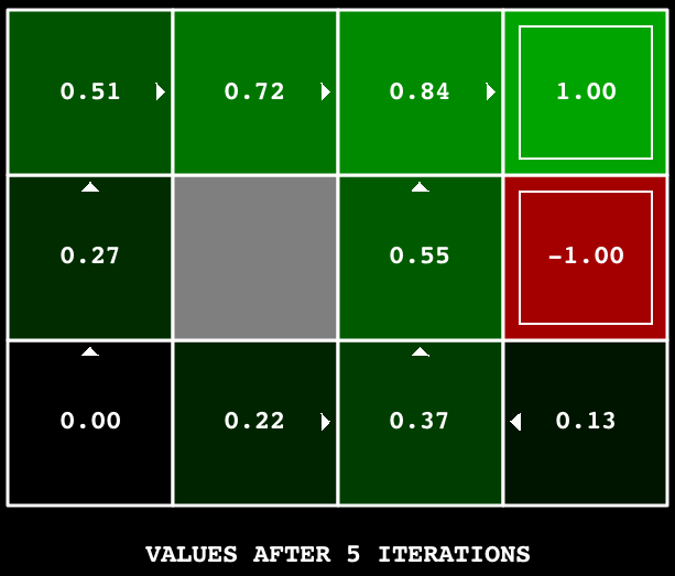
Hint: On the default BookGrid, running
value iteration for 5 iterations should give you this output:
python gridworld.py -a value -i 5
Grading: Your value iteration agent will be graded on a new grid. We will check your values, Q-values, and policies after fixed numbers of iterations and at convergence (e.g. after 100 iterations).
Q2 (1 point): Bridge Crossing Analysis
BridgeGrid is a grid world map with the a
low-reward terminal state and a high-reward terminal state separated by a narrow "bridge", on either side
of
which is a chasm of high negative reward. The agent starts near the low-reward state. With the default
discount of 0.9 and the default noise of 0.2, the optimal policy does not cross the bridge. Change only
ONE
of the discount and noise parameters so that the optimal policy causes the agent to attempt to cross the
bridge. Put your answer in question2() of analysis.py. (Noise refers to how often an agent
ends
up in an unintended successor state when they perform an action.) The default corresponds to:
python gridworld.py -a value -i 100 -g BridgeGrid --discount 0.9 --noise 0.2
Grading: We will check that you only changed one of the given parameters, and that with this change, a correct value iteration agent should cross the bridge. To check your answer, run the autograder:
python autograder.py -q q2
Q3 (6 points): Policies
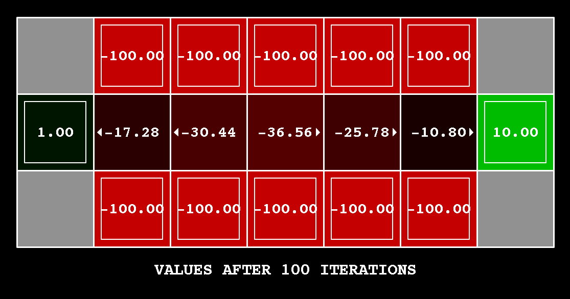
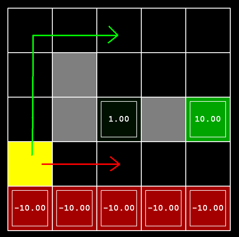
Consider the DiscountGrid layout, shown below.
This grid has two terminal states with positive payoff (in the middle row), a close exit with payoff +1
and
a distant exit with payoff +10. The bottom row of the grid consists of terminal states with negative
payoff
(shown in red); each state in this "cliff" region has payoff -10. The starting state is the yellow square.
We distinguish between two types of paths: (1) paths that "risk the cliff" and travel near the bottom row
of
the grid; these paths are shorter but risk earning a large negative payoff, and are represented by the red
arrow in the figure below. (2) paths that "avoid the cliff" and travel along the top edge of the grid.
These
paths are longer but are less likely to incur huge negative payoffs. These paths are represented by the
green arrow in the figure below.
In this question, you will choose settings of the discount, noise, and living reward parameters for this
MDP to produce optimal policies of several different types. Your setting of the parameter values
for
each part should have the property that, if your agent followed its optimal policy without being subject
to any noise, it would exhibit the given behavior. If a particular behavior is not achieved for
any setting of the parameters, assert that the policy is impossible by returning the string 'NOT POSSIBLE'.
Here are the optimal policy types you should attempt to produce:
- Prefer the close exit (+1), risking the cliff (-10)
- Prefer the close exit (+1), but avoiding the cliff (-10)
- Prefer the distant exit (+10), risking the cliff (-10)
- Prefer the distant exit (+10), avoiding the cliff (-10)
- Avoid both exits and the cliff (so an episode should never terminate)
To see what behavior a set of numbers ends up in, run the following command to see a GUI:
python gridworld.py -g DiscountGrid -a value --discount [YOUR_DISCOUNT] --noise [YOUR_NOISE] --livingReward [YOUR_LIVING_REWARD]
To check your answers, run the autograder:
python autograder.py -q q3
question2a() through question2e() should each return a 3-item tuple of
(discount, noise, living reward) in analysis.py.
Note: You can check your policies in the GUI. For example, using a correct answer to 3(a), the arrow in (0,1) should point east, the arrow in (1,1) should also point east, and the arrow in (2,1) should point north.
Note: On some machines you may not see an arrow. In this case, press a button on the keyboard to switch to qValue display, and mentally calculate the policy by taking the arg max of the available qValues for each state.
Grading: We will check that the desired policy is returned in each case.
Q4 (1 points): Prioritized Sweeping Value Iteration[Extra Credit]
This question is extra credit. We plan to prioritize students who have questions regarding required portions of this assignment in Office Hours.
You will now implement PrioritizedSweepingValueIterationAgent, which has
been
partially specified for you in valueIterationAgents.py.
Prioritized sweeping attempts to focus updates of state values in ways that are likely to change the policy.
For this assignment, you will implement a simplified version of the standard prioritized sweeping
algorithm,
which is described in this paper.
We've adapted this algorithm for our setting. First, we define the predecessors of a state s as all states that have a nonzero probability of
reaching s by taking some action a. Also, theta, which is passed in as a parameter, will
represent our tolerance for error when deciding whether to update the value of a state. Here's the
algorithm
you should follow in your implementation.
- Compute predecessors of all states.
- Initialize an empty priority queue.
- For each non-terminal state
s, do: (note: to make the autograder work for this question, you must iterate over states in the order returned byself.mdp.getStates())- Find the absolute value of the difference between the current value of
sinself.valuesand the highest Q-value across all possible actions froms(this represents what the value should be); call this numberdiff. Do NOT updateself.values[s]in this step. - Push
sinto the priority queue with priority-diff(note that this is negative). We use a negative because the priority queue is a min heap, but we want to prioritize updating states that have a higher error.
- Find the absolute value of the difference between the current value of
- For
iterationin0, 1, 2, ..., self.iterations - 1, do:- If the priority queue is empty, then terminate.
- Pop a state
soff the priority queue. - Update the value of
s(if it is not a terminal state) inself.values. - For each predecessor
pofs, do:- Find the absolute value of the difference between the current value of
pinself.valuesand the highest Q-value across all possible actions fromp(this represents what the value should be); call this numberdiff. Do NOT updateself.values[p]in this step. - If
diff > theta, pushpinto the priority queue with priority-diff(note that this is negative), as long as it does not already exist in the priority queue with equal or lower priority. As before, we use a negative because the priority queue is a min heap, but we want to prioritize updating states that have a higher error.
- Find the absolute value of the difference between the current value of
A couple of important notes on implementation:
- When you compute predecessors of a state, make sure to store them in a set, not a list, to avoid duplicates.
- Please use
util.PriorityQueuein your implementation. Theupdatemethod in this class will likely be useful; look at its documentation.
To test your implementation, run the autograder. It should take about 1 second to run. If it takes much longer, you may run into issues later in the assignment, so make your implementation more efficient now.
python autograder.py -q q4
You can run the PrioritizedSweepingValueIterationAgen in the
Gridworld
using the following command.
python gridworld.py -a priosweepvalue -i 1000
Grading: Your prioritized sweeping value iteration agent will be graded on a new grid. We will check your values, Q-values, and policies after fixed numbers of iterations and at convergence (e.g., after 1000 iterations).
Q5 (5 points): Q-Learning
Note that your value iteration agent does not actually learn from experience. Rather, it ponders its MDP model to arrive at a complete policy before ever interacting with a real environment. When it does interact with the environment, it simply follows the precomputed policy (e.g. it becomes a reflex agent). This distinction may be subtle in a simulated environment like a Gridword, but it's very important in the real world, where the real MDP is not available.
You will now write a Q-learning agent, which does very little on construction, but instead learns by
trial
and error from interactions with the environment through its update(state, action, nextState, reward) method. A
stub of a Q-learner is specified in QLearningAgent
in qlearningAgents.py, and you can select it
with
the option '-a q'. For this question, you must
implement the update, computeValueFromQValues, getQValue, and computeActionFromQValues methods.
Note: For computeActionFromQValues,
you
should break ties randomly for better behavior. The random.choice() function will help. In a particular
state, actions that your agent hasn't seen before still have a Q-value, specifically a Q-value of zero,
and
if all of the actions that your agent has seen before have a negative Q-value, an unseen action may be
optimal.
Important: Make sure that in your computeValueFromQValues and computeActionFromQValues functions, you only access
Q
values by calling getQValue. This abstraction
will
be useful for question 10 when you override getQValue to use features of state-action pairs
rather
than state-action pairs directly.
With the Q-learning update in place, you can watch your Q-learner learn under manual control, using the keyboard:
python gridworld.py -a q -k 5 -m
Recall that -k will control the number of
episodes your agent gets to learn. Watch how the agent learns about the state it was just in, not the one
it
moves to, and "leaves learning in its wake." Hint: to help with debugging, you can turn off noise by using
the --noise 0.0 parameter (though this obviously
makes Q-learning less interesting). If you manually steer Pacman north and then east along the optimal
path
for four episodes, you should see the following Q-values:
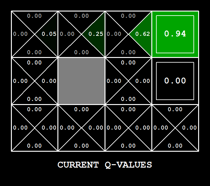
Grading: We will run your Q-learning agent and check that it learns the same Q-values and policy as our reference implementation when each is presented with the same set of examples. To grade your implementation, run the autograder:
python autograder.py -q q5
Q6 (2 points): Epsilon Greedy
Complete your Q-learning agent by implementing epsilon-greedy action selection in getAction, meaning it chooses random actions an
epsilon fraction of the time, and follows its current best Q-values otherwise. Note that choosing a random
action may result in choosing the best action - that is, you should not choose a random sub-optimal
action,
but rather any random legal action.
You can choose an element from a list uniformly at random by calling the random.choice function. You can simulate a binary
variable with probability p of success by using
util.flipCoin(p), which returns True with probability p and False with probability 1-p.
After implementing the getAction method,
observe
the following behavior of the agent in GridWorld
(with epsilon = 0.3).
python gridworld.py -a q -k 100
Your final Q-values should resemble those of your value iteration agent, especially along well-traveled paths. However, your average returns will be lower than the Q-values predict because of the random actions and the initial learning phase.
You can also observe the following simulations for different epsilon values. Does that behavior of the agent match what you expect?
python gridworld.py -a q -k 100 --noise 0.0 -e 0.1
python gridworld.py -a q -k 100 --noise 0.0 -e 0.9
To test your implementation, run the autograder:
python autograder.py -q q6
With no additional code, you should now be able to run a Q-learning crawler robot:
python crawler.py
If this doesn't work, you've probably written some code too specific to the GridWorld problem and you should make it more
general
to all MDPs.
This will invoke the crawling robot from class using your Q-learner. Play around with the various learning parameters to see how they affect the agent's policies and actions. Note that the step delay is a parameter of the simulation, whereas the learning rate and epsilon are parameters of your learning algorithm, and the discount factor is a property of the environment.
Q7 (1 point): Bridge Crossing Revisited
First, train a completely random Q-learner with the default learning rate on the noiseless BridgeGrid for 50 episodes and observe whether it finds the optimal policy.
python gridworld.py -a q -k 50 -n 0 -g BridgeGrid -e 1
Now try the same experiment with an epsilon of 0. Is there an epsilon and a learning rate for which it is
highly likely (greater than 99%) that the optimal policy will be learned after 50 iterations? question8() in analysis.py should return EITHER a 2-item tuple of
(epsilon, learning rate) OR the string 'NOT POSSIBLE' if there is none. Epsilon is
controlled
by -e, learning rate by -l.
Note: Your response should be not depend on the exact tie-breaking mechanism used to choose actions. This means your answer should be correct even if for instance we rotated the entire bridge grid world 90 degrees.
To grade your answer, run the autograder:
python autograder.py -q q7
Q8 (1 point): Q-Learning and Pacman
Time to play some Pacman! Pacman will play games in two phases. In the first phase, training,
Pacman will begin to learn about the values of positions and actions. Because it takes a very long time to
learn accurate Q-values even for tiny grids, Pacman's training games run in quiet mode by default, with no
GUI (or console) display. Once Pacman's training is complete, he will enter testing mode. When
testing, Pacman's self.epsilon and self.alpha will be set to 0.0, effectively stopping
Q-learning and disabling exploration, in order to allow Pacman to exploit his learned policy. Test games
are
shown in the GUI by default. Without any code changes you should be able to run Q-learning Pacman for very
tiny grids as follows:
python pacman.py -p PacmanQAgent -x 2000 -n 2010 -l smallGrid
Note that PacmanQAgent is already defined for
you
in terms of the QLearningAgent you've already
written. PacmanQAgent is only different in that
it
has default learning parameters that are more effective for the Pacman problem (epsilon=0.05, alpha=0.2, gamma=0.8). You will
receive
full credit for this question if the command above works without exceptions and your agent wins at least
80%
of the time. The autograder will run 100 test games after the 2000 training games.
Hint: If your QLearningAgent works for
gridworld.py and crawler.py but does not seem to be learning a good
policy for Pacman on smallGrid, it may be
because
your getAction and/or computeActionFromQValues methods do not in some
cases
properly consider unseen actions. In particular, because unseen actions have by definition a Q-value of
zero, if all of the actions that have been seen have negative Q-values, an unseen action may be optimal.
Beware of the argMax function from util.Counter!
To grade your answer, run:
python autograder.py -q q8
Note: If you want to experiment with learning parameters, you can use the option -a, for example -a epsilon=0.1,alpha=0.3,gamma=0.7. These values
will
then be accessible as self.epsilon, self.gamma and self.alpha inside the agent.
Note: While a total of 2010 games will be played, the first 2000 games will not be displayed
because of the option -x 2000, which designates
the first 2000 games for training (no output). Thus, you will only see Pacman play the last 10 of these
games. The number of training games is also passed to your agent as the option numTraining.
Note: If you want to watch 10 training games to see what's going on, use the command:
python pacman.py -p PacmanQAgent -n 10 -l smallGrid -a numTraining=10
During training, you will see output every 100 games with statistics about how Pacman is faring. Epsilon is positive during training, so Pacman will play poorly even after having learned a good policy: this is because he occasionally makes a random exploratory move into a ghost. As a benchmark, it should take between 1000 and 1400 games before Pacman's rewards for a 100 episode segment becomes positive, reflecting that he's started winning more than losing. By the end of training, it should remain positive and be fairly high (between 100 and 350).
Make sure you understand what is happening here: the MDP state is the exact board configuration facing Pacman, with the now complex transitions describing an entire ply of change to that state. The intermediate game configurations in which Pacman has moved but the ghosts have not replied are not MDP states, but are bundled in to the transitions.
Once Pacman is done training, he should win very reliably in test games (at least 90% of the time), since now he is exploiting his learned policy.
However, you will find that training the same agent on the seemingly simple mediumGrid does not work well. In our
implementation,
Pacman's average training rewards remain negative throughout training. At test time, he plays badly,
probably losing all of his test games. Training will also take a long time, despite its ineffectiveness.
Pacman fails to win on larger layouts because each board configuration is a separate state with separate Q-values. He has no way to generalize that running into a ghost is bad for all positions. Obviously, this approach will not scale.
Q9 (4 points): Approximate Q-Learning
Implement an approximate Q-learning agent that learns weights for features of states, where many states
might share the same features. Write your implementation in ApproximateQAgent class in qlearningAgents.py, which is a subclass of PacmanQAgent.
Note: Approximate Q-learning assumes the existence of a feature function \(f(s,a)\) over state
and
action pairs, which yields a vector \([f_1(s,a), \dots, f_i(s,a), \dots, f_n(s,a)]\) of feature values. We
provide feature functions for you in featureExtractors.py. Feature vectors are util.Counter (like a dictionary) objects containing
the non-zero pairs of features and values; all omitted features have value zero. So, instead of an vector
where the index in the vector defines which feature is which, we have the keys in the dictionary define
the
idenity of the feature.
The approximate Q-function takes the following form:
\[Q(s,a)=\sum_{i=1}^n f_i(s,a) w_i\]where each weight \(w_i\) is associated with a particular feature \(f_i(s,a)\). In your code, you should implement the weight vector as a dictionary mapping features (which the feature extractors will return) to weight values. You will update your weight vectors similarly to how you updated Q-values:
\[w_i \leftarrow w_i + \alpha \cdot \text{difference} \cdot f_i(s,a)\] \[\text{difference} = \left( r + \gamma \max_{a'}Q(s',a') \right) - Q(s,a)\]Note that the \(\text{difference}\) term is the same as in normal Q-learning, and \(r\) is the experienced reward.
By default, ApproximateQAgent uses the IdentityExtractor, which assigns a single feature to
every (state,action) pair. With this feature
extractor, your approximate Q-learning agent should work identically to PacmanQAgent. You can test this with the following
command:
python pacman.py -p ApproximateQAgent -x 2000 -n 2010 -l smallGrid
Important: ApproximateQAgent is a
subclass of QLearningAgent, and it therefore
shares several methods like getAction. Make sure
that your methods in QLearningAgent call getQValue instead of accessing Q-values directly, so
that when you override getQValue in your
approximate agent, the new approximate q-values are used to compute actions.
Once you're confident that your approximate learner works correctly with the identity features, run your approximate Q-learning agent with our custom feature extractor, which can learn to win with ease:
python pacman.py -p ApproximateQAgent -a extractor=SimpleExtractor -x 50 -n 60 -l mediumGrid
Even much larger layouts should be no problem for your ApproximateQAgent (warning: this may take a
few minutes to train):
python pacman.py -p ApproximateQAgent -a extractor=SimpleExtractor -x 50 -n 60 -l mediumClassic
If you have no errors, your approximate Q-learning agent should win almost every time with these simple features, even with only 50 training games.
Grading: We will run your approximate Q-learning agent and check that it learns the same Q-values and feature weights as our reference implementation when each is presented with the same set of examples. To grade your implementation, run the autograder:
python autograder.py -q q9
Congratulations! You have a learning Pacman agent!
Submission
In order to submit your solutions, please upload the following files to Canvas -> Assignments -> Assignment 3: Reinforcement Learning:valueIterationAgents.py,
qlearningAgents.py, and analysis.py. Please upload the files in a single
zip
file
named <your
UIN>.zip.
Pacman uses probabilistic inference on Bayes Nets and the forward algorithm and particle sampling in a Hidden Markov Model to find ghosts given noisy readings of distances to them.
Pacman spends his life running from ghosts, but things were not always so. Legend has it that many years ago, Pacman's great grandfather Grandpac learned to hunt ghosts for sport. However, he was blinded by his power and could only track ghosts by their banging and clanging.
In this assignment, you will design Pacman agents that use sensors to locate and eat invisible ghosts. You'll advance from locating single, stationary ghosts to hunting packs of multiple moving ghosts with ruthless efficiency.
This assignment includes an autograder for you to grade your answers on your machine. This can be run on all questions with the command:
python autograder.py
It can be run for one particular question, such as q2, by:
python autograder.py -q q2
It can be run for one particular test by commands of the form:
python autograder.py -t test_cases/q1/1-ObsProb
The code for this assignment contains the following files, available as a zip archive.
| Files you'll edit: | |
bustersAgents.py |
Agents for playing the Ghostbusters variant of Pacman. |
inference.py |
Code for tracking ghosts over time using their sounds. |
factorOperations.py |
Operations to compute new joint or magrinalized probability tables. |
| Files you might want to look at: | |
bayesNet.py |
The BayesNet and Factor classes. |
| Supporting files you can ignore: | |
busters.py |
The main entry to Ghostbusters (replacing Pacman.py). |
bustersGhostAgents.py |
New ghost agents for Ghostbusters. |
distanceCalculator.py |
Computes maze distances, caches results to avoid re-computing. |
game.py |
Inner workings and helper classes for Pacman. |
ghostAgents.py |
Agents to control ghosts. |
graphicsDisplay.py |
Graphics for Pacman. |
graphicsUtils.py |
Support for Pacman graphics. |
keyboardAgents.py |
Keyboard interfaces to control Pacman. |
layout.py |
Code for reading layout files and storing their contents. |
util.py |
Utility functions. |
Files to Edit and Submit: You will fill in portions of bustersAgents.py, inference.py, and factorOperations.py during the assignment. Once you
have completed the assignment, you will submit these files to Gradescope (for instance, you can upload all
.py files in the folder). Please do not change the
other files in this distribution.
Evaluation: Your code will be autograded for technical correctness. Please do not change the names of any provided functions or classes within the code, or you will wreak havoc on the autograder. However, the correctness of your implementation – not the autograder's judgements – will be the final judge of your score. If necessary, we will review and grade assignments individually to ensure that you receive due credit for your work.
Academic Dishonesty: We will be checking your code against other submissions in the class for logical redundancy. If you copy someone else's code and submit it with minor changes, we will know. These cheat detectors are quite hard to fool, so please don't try. We trust you all to submit your own work only; please don't let us down. If you do, we will pursue the strongest consequences available to us.
Getting Help: You are not alone! If you find yourself stuck on something, contact the course staff for help. Office hours and the course Campuswire are there for your support; please use them. We want these assignments to be rewarding and instructional, not frustrating and demoralizing.
Discussion: Please be careful not to post spoilers.
Ghostbusters and Bayes Nets
In the CSCE-420 version of Ghostbusters, the goal is to hunt down scared but invisible ghosts. Pacman, ever resourceful, is equipped with sonar (ears) that provides noisy readings of the Manhattan distance to each ghost. The game ends when Pacman has eaten all the ghosts. To start, try playing a game yourself using the keyboard.
python busters.py
The blocks of color indicate where the each ghost could possibly be, given the noisy distance readings provided to Pacman. The noisy distances at the bottom of the display are always non-negative, and always within 7 of the true distance. The probability of a distance reading decreases exponentially with its difference from the true distance.
Your primary task in this assignment is to implement inference to track the ghosts. For the keyboard based game above, a crude form of inference was implemented for you by default: all squares in which a ghost could possibly be are shaded by the color of the ghost. Naturally, we want a better estimate of the ghost's position. Fortunately, Bayes Nets provide us with powerful tools for making the most of the information we have. Throughout the rest of this assignment, you will implement algorithms for performing both exact and approximate inference using Bayes Nets. The assignment is challenging, so we do encouarge you to start early and seek help when necessary.
While watching and debugging your code with the autograder, it will be helpful to have some understanding
of what the autograder is doing. There are 2 types of tests in this assignment, as differentiated by their
.test files found in the subdirectories of the
test_cases folder. For tests of class DoubleInferenceAgentTest, you will see visualizations
of the inference distributions generated by your code, but all Pacman actions will be pre-selected according
to the actions of the staff implementation. This is necessary to allow comparision of your distributions
with the staff's distributions. The second type of test is GameScoreTest, in which your BustersAgent will actually select actions for Pacman
and you will watch your Pacman play and win games.
For this assignment, it is possible sometimes for the autograder to time out if running the tests with
graphics. To accurately determine whether or not your code is efficient enough, you should run the tests
with the --no-graphics flag. If the autograder
passes with this flag, then you will receive full points, even if the autograder times out with graphics.
Bayes Nets and Factors
First, take a look at bayesNet.py to see the
classes you'll be working with – BayesNet and
Factor. You can also run this file to see an
example BayesNet and associated Factors: python bayesNet.py.
You should look at the printStarterBayesNet
function – there are helpful comments that can make your life much easier later on.
The Bayes Net created in this function is shown below:
(Raining –> Traffic <– Ballgame)
A summary of the terminology is given below:
- Bayes Net: This is a representation of a probabilistic model as a directed acyclic graph and a set of conditional probability tables, one for each variable, as shown in lecture. The Traffic Bayes Net above is an example.
- Factor: This stores a table of probabilities, although the sum of the entries in the table is not necessarily 1. A factor is of the general form \(f(X_1, \dots, X_m,y_1, \dots,y_n\mid Z_1, \dots, Z_p, w_1, \dots, w_q)\). Recall that lower case variables have already been assigned. For each possible assignment of values to the \(X_i\) and \(Z_j\) variables, the factor stores a single number. The \(Z_j\) and \(w_k\) variables are said to be conditioned while the \(X_i\) and \(y_l\) variables are unconditioned.
- Conditional Probability Table (CPT): This is a factor satisfying two
properties:
- Its entries must sum to 1 for each assignment of the conditional variables.
- There is exactly one unconditioned variable. The Traffic Bayes Net stores the following CPTs: \(P(Raining)\), \(P(Ballgame)\), \(P(Traffic\mid Ballgame,Raining)\).
Q1 (2 points): Bayes Net Structure
Implement the constructBayesNet function in inference.py. It constructs an empty Bayes Net with
the structure described below. A Bayes Net is incomplete without the actual probabilities, but factors are
defined and assigned by staff code separately; you don't need to worry about it. If you are curious, you can
take a look at an example of how it works in printStarterBayesNet in bayesNet.py. Reading this function can also be helpful
for doing this question.
The simplified ghost hunting world is generated according to the following Bayes net:
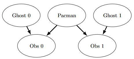
Don't worry if this looks complicated! We'll take it step by step. As described in the code for constructBayesNet, we build the empty structure by
listing all of the variables, their values, and the edges between them. This figure shows the variables and
the edges, but what about their domains?
- Add variables and edges based on the diagram.
- Pacman and the two ghosts can be anywhere in the grid (we ignore walls for this). Add all possible position tuples for these.
- Observations here are non-negative, equal to Manhattan distances of Pacman to ghosts \(\pm\) noise.
Grading: To test and debug your code, run
python autograder.py -q q1
Q2 (3 points): Join Factors
Implement the joinFactors function in factorOperations.py. It takes in a list of Factors and returns a new Factor whose probability entries are the product of
the corresponding rows of the input Factors.
joinFactors can be used as the product rule, for
example, if we have a factor of the form \(P(X\mid Y)\) and another factor of the form \(P(Y)\), then
joining these factors will yield \(P(X,Y)\). So, joinFactors allows us to incorporate probabilities for
conditioned variables (in this case, \(Y\)). However, you should not assume that joinFactors is called on probability tables – it is
possible to call joinFactors on Factors whose rows do not sum to 1.
Grading: To test and debug your code, run
python autograder.py -q q2
It may be useful to run specific tests during debugging, to see only one set of factors print out. For example, to only run the first test, run:
python autograder.py -t test_cases/q2/1-product-rule
Hints and Observations:
- Your
joinFactorsshould return a newFactor. - Here are some examples of what
joinFactorscan do:joinFactors\((P(X \mid Y), P(Y)) = P(X,Y)\)joinFactors\((P(V,W \mid X,Y,Z), P(X,Y \mid Z)) = P(V,W,X,Y \mid Z)\)joinFactors\((P(X \mid Y,Z), P(Y)) = P(X,Y \mid Z)\)joinFactors\((P(V \mid W), P(X \mid Y), P(Z)) = P(V,X,Z \mid W,Y)\)
- For a general
joinFactorsoperation, which variables are unconditioned in the returnedFactor? Which variables are conditioned? Factors store avariableDomainsDict, which maps each variable to a list of values that it can take on (its domain). AFactorgets itsvariableDomainsDictfrom theBayesNetfrom which it was instantiated. As a result, it contains all the variables of theBayesNet, not only the unconditioned and conditioned variables used in theFactor. For this problem, you may assume that all the inputFactors have come from the sameBayesNet, and so theirvariableDomainsDictsare all the same.
Q3 (2 points): Eliminate (not ghosts yet)
Implement the eliminate function in factorOperations.py. It takes a Factor and a variable to eliminate and returns a new
Factor that does not contain that variable. This
corresponds to summing all of the entries in the Factor which only differ in the value of the variable
being eliminated.
Grading: To test and debug your code, run
python autograder.py -q q3
It may be useful to run specific tests during debugging, to see only one set of factors print out. For example, to only run the first test, run:
python autograder.py -t test_cases/q3/1-simple-eliminate
Hints and Observations:
- Your eliminate should return a new
Factor. eliminatecan be used to marginalize variables from probability tables. For example:eliminate\((P(X,Y \mid Z), Y) = P(X \mid Z)\)eliminate\((P(X,Y \mid Z), X) = P(Y \mid Z)\)
- For a general eliminate operation, which variables are unconditioned in the returned Factor? Which variables are conditioned?
- Remember that
Factors store thevariableDomainsDictof the originalBayesNet, and not only the unconditioned and conditioned variables that they use. As a result, the returnedFactorshould have the samevariableDomainsDictas the inputFactor.
Q4 (2 points): Variable Elimination
Implement the inferenceByVariableElimination
function in inference.py. It answers a
probabilistic query, which is represented using a BayesNet, a list of query variables, and the evidence.
Grading: To test and debug your code, run
python autograder.py -q q4
It may be useful to run specific tests during debugging, to see only one set of factors print out. For example, to only run the first test, run:
python autograder.py -t test_cases/q4/1-disconnected-eliminate
Hints and Observations:
- The algorithm should iterate over hidden variables in elimination order, performing joining over and eliminating that variable, until the only the query and evidence variables remain.
- The sum of the probabilities in your output factor should sum to 1 (so that it is a true conditional probability, conditioned on the evidence).
- Look at the
inferenceByEnumerationfunction ininference.pyfor an example on how to use the desired functions. (Reminder: Inference by enumeration first joins over all the variables and then eliminates all the hidden variables. In contrast, variable elimination interleaves join and eliminate by iterating over all the hidden variables and perform a join and eliminate on a single hidden variable before moving on to the next hidden variable.) - You will need to take care of the special case where a factor you have joined only has one unconditioned variable (the docstring specifies what to do in greater detail).
Question 5a: DiscreteDistribution Class
Unfortunately, having timesteps will grow our graph far too much for variable elimination to be viable. Instead, we will use the Forward Algorithm for HMM's for exact inference, and Particle Filtering for even faster but approximate inference.
For the rest of the assignment, we will be using the DiscreteDistribution class defined in inference.py to model belief distributions and weight
distributions. This class is an extension of the built-in Python dictionary class, where the keys are the
different discrete elements of our distribution, and the corresponding values are proportional to the belief
or weight that the distribution assigns that element. This question asks you to fill in the missing parts of
this class, which will be crucial for later questions (even though this question itself is worth no points).
First, fill in the normalize method, which
normalizes the values in the distribution to sum to one, but keeps the proportions of the values the same.
Use the total method to find the sum of the values
in the distribution. For an empty distribution or a distribution where all of the values are zero, do
nothing. Note that this method modifies the distribution directly, rather than returning a new distribution.
Second, fill in the sample method, which draws a
sample from the distribution, where the probability that a key is sampled is proportional to its
corresponding value. Assume that the distribution is not empty, and not all of the values are zero. Note
that the distribution does not necessarily have to be normalized prior to calling this method. You may find
Python's built-in random.random() function useful
for this question.
Q5b (1 point): Observation Probability
In this question, you will implement the getObservationProb method in the InferenceModule base class in inference.py. This method takes in an observation
(which is a noisy reading of the distance to the ghost), Pacman's position, the ghost's position, and the
position of the ghost's jail, and returns the probability of the noisy distance reading given Pacman's
position and the ghost's position. In other words, we want to return \(P(noisyDistance \mid pacmanPosition,
ghostPosition)\).
The distance sensor has a probability distribution over distance readings given the true distance from
Pacman to the ghost. This distribution is modeled by the function busters.getObservationProbability(noisyDistance, trueDistance),
which returns \(P(noisyDistance \mid trueDistance)\) and is provided for you. You should use this function
to help you solve the problem, and use the provided manhattanDistance function to find the distance
between Pacman's location and the ghost's location.
However, there is the special case of jail that we have to handle as well. Specifically, when we capture a
ghost and send it to the jail location, our distance sensor deterministically returns None, and nothing else (observation = None if and only if ghost is in jail). One consequence
of this is that if the ghost's position is the jail position, then the observation is None with probability 1, and everything else with
probability 0. Make sure you handle this special case in your implementation; we effectively have a
different set of rules for whenever ghost is in jail, as well as whenever observation is None.
To test your code and run the autograder for this question:
python autograder.py -q q5
Q6 (2 points): Exact Inference Observation
In this question, you will implement the observeUpdate method in ExactInference class of inference.py to correctly update the agent's belief
distribution over ghost positions given an observation from Pacman's sensors. You are implementing the
online belief update for observing new evidence. The observeUpdate method should, for this problem, update
the belief at every position on the map after receiving a sensor reading. You should iterate your updates
over the variable self.allPositions which includes
all legal positions plus the special jail position. Beliefs represent the probability that the ghost is at a
particular location, and are stored as a DiscreteDistribution object in a field called self.beliefs, which you should update.
Before typing any code, write down the equation of the inference problem you are trying to solve. You
should use the function self.getObservationProb
that you wrote in the last question, which returns the probability of an observation given Pacman's
position, a potential ghost position, and the jail position. You can obtain Pacman's position using gameState.getPacmanPosition(), and the jail position
using self.getJailPosition().
In the Pacman display, high posterior beliefs are represented by bright colors, while low beliefs are represented by dim colors. You should start with a large cloud of belief that shrinks over time as more evidence accumulates. As you watch the test cases, be sure that you understand how the squares converge to their final coloring.
Note: your busters agents have a separate inference module for each ghost they are tracking. That's why if
you print an observation inside the observeUpdate
function, you'll only see a single number even though there may be multiple ghosts on the board.
To run the autograder for this question and visualize the output:
python autograder.py -q q6
If you want to run this test (or any of the other tests) without graphics you can add the following flag:
python autograder.py -q q6 --no-graphics
Q7 (2 points): Exact Inference with Time Elapse
In the previous question you implemented belief updates for Pacman based on his observations. Fortunately, Pacman's observations are not his only source of knowledge about where a ghost may be. Pacman also has knowledge about the ways that a ghost may move; namely that the ghost can not move through a wall or more than one space in one time step.
To understand why this is useful to Pacman, consider the following scenario in which there is Pacman and one Ghost. Pacman receives many observations which indicate the ghost is very near, but then one which indicates the ghost is very far. The reading indicating the ghost is very far is likely to be the result of a buggy sensor. Pacman's prior knowledge of how the ghost may move will decrease the impact of this reading since Pacman knows the ghost could not move so far in only one move.
In this question, you will implement the elapseTime method in ExactInference. The elapseTime step should, for this problem, update the
belief at every position on the map after one time step elapsing. Your agent has access to the action
distribution for the ghost through self.getPositionDistribution. In order to obtain the
distribution over new positions for the ghost, given its previous position, use this line of code:
newPosDist = self.getPositionDistribution(gameState, oldPos)
Where oldPos refers to the previous ghost
position. newPosDist is a DiscreteDistribution object, where for each position
p in self.allPositions, newPosDist[p] is the probability that the ghost is at
position p at time t + 1, given that the ghost is at position oldPos at time t. Note that this call can be fairly expensive, so if
your code is timing out, one thing to think about is whether or not you can reduce the number of calls to
self.getPositionDistribution.
Before typing any code, write down the equation of the inference problem you are trying to solve. In order to test your predict implementation separately from your update implementation in the previous question, this question will not make use of your update implementation.
Since Pacman is not observing the ghost's actions, these actions will not impact Pacman's beliefs. Over time, Pacman's beliefs will come to reflect places on the board where he believes ghosts are most likely to be given the geometry of the board and ghosts' possible legal moves, which Pacman already knows.
For the tests in this question we will sometimes use a ghost with random movements and other times we will
use the GoSouthGhost. This ghost tends to move
south so over time, and without any observations, Pacman's belief distribution should begin to focus around
the bottom of the board. To see which ghost is used for each test case you can look in the .test files.
The below diagram shows what the Bayes Net/ Hidden Markov model for what is happening. Still, you should
rely on the above description for implementation because some parts are implemented for you (i.e. getPositionDistribution is abstracted to be
\(P(G_{t+1} \mid gameState, G_t))\).
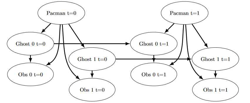
To run the autograder for this question and visualize the output:
python autograder.py -q q7
If you want to run this test (or any of the other tests) without graphics you can add the following flag:
python autograder.py -q q7 --no-graphics
As you watch the autograder output, remember that lighter squares indicate that pacman believes a ghost is more likely to occupy that location, and darker squares indicate a ghost is less likely to occupy that location. For which of the test cases do you notice differences emerging in the shading of the squares? Can you explain why some squares get lighter and some squares get darker?
Q8 (1 point): Exact Inference Full Test
Now that Pacman knows how to use both his prior knowledge and his observations when figuring out where a
ghost is, he is ready to hunt down ghosts on his own. We will use your observeUpdate and elapseTime implementations together to keep an updated
belief distribution, and your simple greedy agent will choose an action based on the latest ditsibutions at
each time step. In the simple greedy strategy, Pacman assumes that each ghost is in its most likely position
according to his beliefs, then moves toward the closest ghost. Up to this point, Pacman has moved by
randomly selecting a valid action.
Implement the chooseAction method in GreedyBustersAgent in bustersAgents.py. Your agent should first find the
most likely position of each remaining uncaptured ghost, then choose an action that minimizes the maze
distance to the closest ghost.
To find the maze distance between any two positions pos1 and pos2, use self.distancer.getDistance(pos1, pos2). To find the
successor position of a position after an action:
successorPosition = Actions.getSuccessor(position, action)
You are provided with livingGhostPositionDistributions, a list of DiscreteDistribution objects representing the position
belief distributions for each of the ghosts that are still uncaptured.
If correctly implemented, your agent should win the game in q8/3-gameScoreTest with a score greater than 700 at
least 8 out of 10 times. Note: the autograder will also check the correctness of your inference directly,
but the outcome of games is a reasonable sanity check.
We can represent how our greedy agent works with the following modification to the previous diagram:
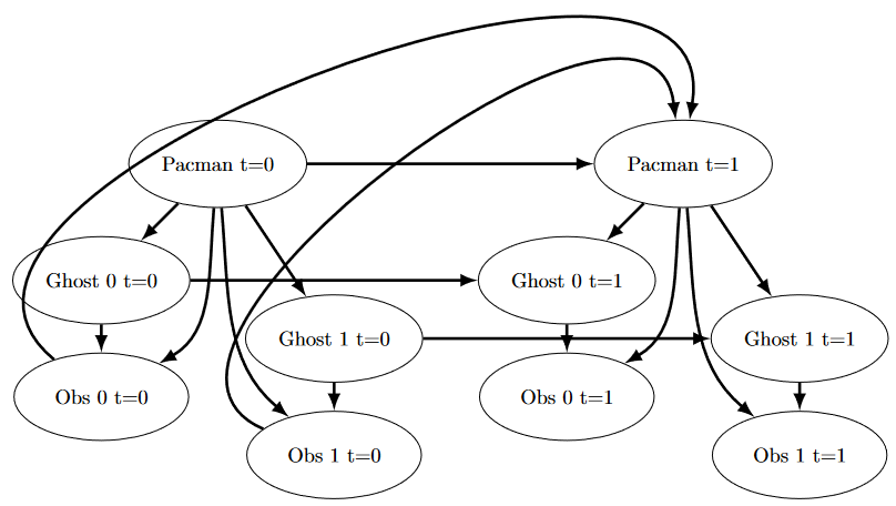
Bayes net diagram
To run the autograder for this question and visualize the output:
python autograder.py -q q8
If you want to run this test (or any of the other tests) without graphics you can add the following flag:
python autograder.py -q q8 --no-graphics
Q9 (1 point): Approximate Inference Initialization and Beliefs
Approximate inference is very trendy among ghost hunters this season. For the next few questions, you will implement a particle filtering algorithm for tracking a single ghost.
First, implement the functions initializeUniformly and getBeliefDistribution in the ParticleFilter class in inference.py. A particle (sample) is a ghost position
in this inference problem. Note that, for initialization, particles should be evenly (not randomly)
distributed across legal positions in order to ensure a uniform prior. We recommend thinking about how the
mod operator is useful for initializeUniformly.
Note that the variable you store your particles in must be a list. A list is simply a collection of
unweighted variables (positions in this case). Storing your particles as any other data type, such as a
dictionary, is incorrect and will produce errors. The getBeliefDistribution method then takes the list of
particles and converts it into a DiscreteDistribution object.
To test your code and run the autograder for this question:
python autograder.py -q q9
Q10 (2 points): Approximate Inference Observation
Next, we will implement the observeUpdate method
in the ParticleFilter class in inference.py. This method constructs a weight
distribution over self.particles where the weight
of a particle is the probability of the observation given Pacman's position and that particle location.
Then, we resample from this weighted distribution to construct our new list of particles.
You should again use the function self.getObservationProb to find the probability of an
observation given Pacman's position, a potential ghost position, and the jail position. The sample method of
the DiscreteDistribution class will also be
useful. As a reminder, you can obtain Pacman's position using gameState.getPacmanPosition(), and the jail position
using self.getJailPosition().
There is one special case that a correct implementation must handle. When all particles receive zero
weight, the list of particles should be reinitialized by calling initializeUniformly. The total method of the DiscreteDistribution may be useful.
To run the autograder for this question and visualize the output:
python autograder.py -q q10
If you want to run this test (or any of the other tests) without graphics you can add the following flag:
python autograder.py -q q10 --no-graphics
Q11 (2 points): Approximate Inference with Time Elapse
Implement the elapseTime function in the ParticleFilter class in inference.py. This function should construct a new
list of particles that corresponds to each existing particle in self.particles advancing a time step, and then assign
this new list back to self.particles. When
complete, you should be able to track ghosts nearly as effectively as with exact inference.
Note that in this question, we will test both the elapseTime function in isolation, as well as the full
implementation of the particle filter combining elapseTime and observe.
As in the elapseTime method of the ExactInference class, you should use:
newPosDist = self.getPositionDistribution(gameState, oldPos)
This line of code obtains the distribution over new positions for the ghost, given its previous position
(oldPos). The sample method of the DiscreteDistribution class will also be useful.
To run the autograder for this question and visualize the output:
python autograder.py -q q11
If you want to run this test (or any of the other tests) without graphics you can add the following flag:
python autograder.py -q q11 --no-graphics
Note that even with no graphics, this test may take several minutes to run.
Submission
In order to submit your solutions, please upload the following files to Canvas -> Assignments ->
Assignment 4: Bayes Nets and HMMs: bustersAgents.py,
inference.py, and factorOperations.py. Please upload the files in a single
zip
file
named <your
UIN>.zip.
Students implement the perceptron algorithm, neural network, and recurrent nn models, and apply the models to several tasks including digit classification and language identification.
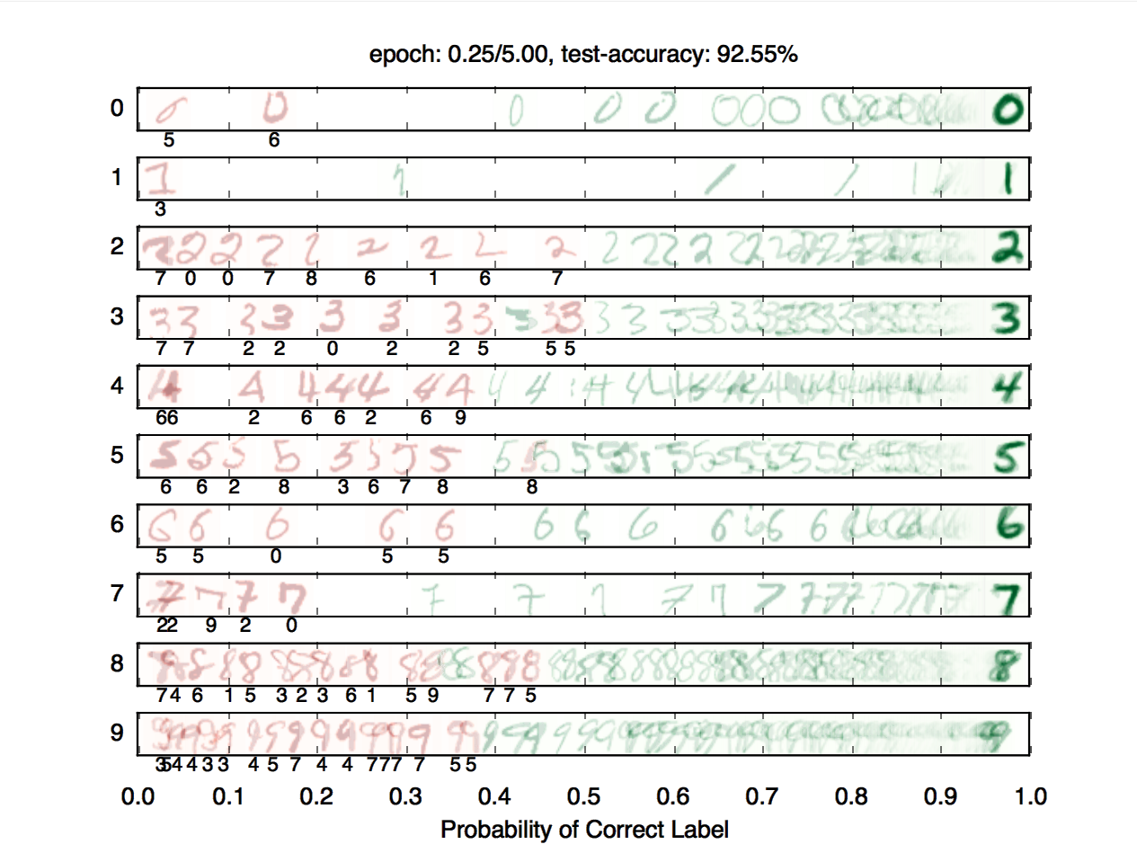
Introduction
This assignment will be an introduction to machine learning; you will build a neural network to classify digits, and more!
The code for this assignment contains the following files, available as a zip archive.
| Files you'll edit: | |
models.py |
Perceptron and neural network models for a variety of applications. |
| Files you might want to look at: | |
nn.py |
Neural network mini-library. |
| Supporting files you can ignore: | |
autograder.py |
Assignment autograder. |
backend.py |
Backend code for various machine learning tasks. |
data |
Datasets for digit classification and language identification. |
Files to Edit and Submit: You will fill in portions of models.py during the assignment. Once you have
completed the assignment, you will submit these files to Canvsas (for instance, you can upload all .py files in the folder). Please do not change the
other files in this distribution.
Evaluation: Your code will be autograded for technical correctness. Please do not change the names of any provided functions or classes within the code, or you will wreak havoc on the autograder. However, the correctness of your implementation -- not the autograder's judgements -- will be the final judge of your score. If necessary, we will review and grade assignments individually to ensure that you receive due credit for your work.
Academic Dishonesty: We will be checking your code against other submissions in the class for logical redundancy. If you copy someone else's code and submit it with minor changes, we will know. These cheat detectors are quite hard to fool, so please don't try. We trust you all to submit your own work only; please don't let us down. If you do, we will pursue the strongest consequences available to us.
Getting Help: You are not alone! If you find yourself stuck on something, contact the course staff for help. Office hours, section, and the discussion forum are there for your support; please use them. If you can't make our office hours, let us know and we will schedule more. We want these projects to be rewarding and instructional, not frustrating and demoralizing.
Discussion: Please be careful not to post spoilers.
Installation
If the following runs and you see the below window pop up where a line segment spins in a circle, you can skip this section. You should use the conda environment for this since conda comes with the libraries we need.
python autograder.py --check-dependencies
For this assignment, you will need to install the following two libraries:
- numpy, which provides support for fast, large multi-dimensional arrays.
- matplotlib, a 2D plotting library.
If you have a conda environment, you can install both packages on the command line by running:
conda activate [your environment name]
pip install numpy
  pip install matplotlib
You will not be using these libraries directly, but they are required in order to run the provided code and autograder.
If your setup is different, you can refer to numpy and matplotlib installation instructions. You can use
either pip or conda to install the packages; pip works both inside and outside of conda
environments.
After installing, try the dependency check.
Provided Code (Part I)
For this assignment, you have been provided with a neural network mini-library (nn.py) and a collection of datasets (backend.py).
The library in nn.py defines a collection of node
objects. Each node represents a real number or a matrix of real numbers. Operations on node objects are
optimized to work faster than using Python's built-in types (such as lists).
Here are a few of the provided node types:
nn.Constantrepresents a matrix (2D array) of floating point numbers. It is typically used to represent input features or target outputs/labels. Instances of this type will be provided to you by other functions in the API; you will not need to construct them directly.nn.Parameterrepresents a trainable parameter of a perceptron or neural network.nn.DotProductcomputes a dot product between its inputs. Additional provided functions:
nn.as_scalar can extract a Python floating-point
number from a node.
When training a perceptron or neural network, you will be passed a dataset object. You can retrieve batches
of training examples by calling dataset.iterate_once(batch_size):
for x, y in dataset.iterate_once(batch_size):
    ...
For example, let's extract a batch of size 1 (i.e., a single training example) from the perceptron training data:
>>> batch_size = 1
>>> for x, y in dataset.iterate_once(batch_size):
...     print(x)
...     print(y)
...     break
...
<Constant shape=1x3 at 0x11a8856a0>
<Constant shape=1x1 at 0x11a89efd0>
The input features x and the correct label y are provided in the form of nn.Constant nodes. The shape of x will be batch_size x num_features, and the shape of y is batch_size x num_outputs. So, each row of x is a point/ sample, and a column is the same feature
of some samples. Here is an example of computing a dot product of x with itself, first as a node and then as a Python
number.
>>> nn.DotProduct(x, x)
<DotProduct shape=1x1 at 0x11a89edd8>
>>> nn.as_scalar(nn.DotProduct(x, x))
1.9756581717465536
Finally, here are some formulations of matrix multiplication (you can do some examples by hand to verify this). Let \(\mathbf A\) be an \(m \times n\) matrix and \(\mathbf B\) be \(n \times p\); matrix multiplication works as follows:
\[\mathbf A\mathbf B=\begin{bmatrix} \vec A_0^T \\ \vec A_1^T \\ \cdots \\ \vec A_{m-1}^T \end{bmatrix} \mathbf B =\begin{bmatrix} \vec A_0^T \mathbf B \\ \vec A_1^T \mathbf B \\ \cdots \\ \vec A_{m-1}^T \mathbf B \end{bmatrix} \qquad \mathbf A\mathbf B=\mathbf A\begin{bmatrix} \vec B_0 & \vec B_1 & \cdots & \vec B_{p-1} \end{bmatrix} =\begin{bmatrix} \mathbf A\vec B_0 & \mathbf A\vec B_1 & \cdots & \mathbf A\vec B_{p-1} \end{bmatrix}\]- As a sanity check, the dimensions are what we expect them to be, and the inner dimension of \(n\) is preserved for any remaining matrix multiplications.
- This is useful to see what happens when we multiply a batch matrix \(X\) by a weight matrix \(W\), we are just multiplying each sample one at a time by the entire weight matrix via the first formulation. Within each sample times weights, we are just getting different linear combinations of the sample to go to each result column via the second formulation. Note that as long as the dimensiosn match, \(A\) can be a row vector and \(B\) a column vector.
Q1 (6 points): Perceptron
Before starting this part, be sure you have numpy
and matplotlib installed!
In this part, you will implement a binary perceptron. Your task will be to complete the implementation of
the PerceptronModel class in models.py.
For the perceptron, the output labels will be either 1 or -1, meaning that data points (x, y) from the dataset will have y be a nn.Constant node that contains either 1 or -1 as its entries.
We have already initialized the perceptron weights self.w to be a 1 by dimensions parameter node. The provided code will
include a bias feature inside x when needed, so
you will not need a separate parameter for the bias.
Your tasks are to:
- Implement the
run(self, x)method. This should compute the dot product of the stored weight vector and the given input, returning annn.DotProductobject. - Implement
get_prediction(self, x), which should return1if the dot product is non-negative or-1otherwise. You should usenn.as_scalarto convert a scalarNodeinto a Python floating-point number. - Write the
train(self)method. This should repeatedly loop over the data set and make updates on examples that are misclassified. Use theupdatemethod of thenn.Parameterclass to update the weights. When an entire pass over the data set is completed without making any mistakes, 100% training accuracy has been achieved, and training can terminate. - In this assignment, the only way to change the value of a parameter is by calling
parameter.update(direction, multiplier), which will perform the update to the weights:
The direction argument is a Node with the same shape as the parameter, and the
multiplier argument is a Python scalar.
Additionally, use iterate_once to loop over the
dataset; see Provided Code (Part I) for usage.
To test your implementation, run the autograder:
python autograder.py -q q1
Note: the autograder should take at most 20 seconds or so to run for a correct implementation. If the autograder is taking forever to run, your code probably has a bug.
Neural Network Tips
In the remaining parts of the assignment, you will implement the following models:
Building Neural Nets
Throughout the applications portion of the assignment, you'll use the framework provided in nn.py to create neural networks to solve a variety of
machine learning problems. A simple neural network has linear layers, where each linear layer performs a
linear operation (just like perceptron). Linear layers are separated by a non-linearity, which
allows the network to approximate general functions. We'll use the ReLU operation for our non-linearity,
defined as \(\text{relu}(x)=\max(x,0)\). For example, a simple one hidden layer/ two linear layers neural
network for mapping an input row vector \(\mathbf x\) to an output vector \(\mathbf f(\mathbf x)\) would be
given by the function:
where we have parameter matrices \(\mathbf{W_1}\) and \(\mathbf{W_2}\) and parameter vectors \(\mathbf{b_1}\) and \(\mathbf{b_2}\) to learn during gradient descent. \(\mathbf{W_1}\) will be an \(i \times h\) matrix, where \(i\) is the dimension of our input vectors \(\mathbf{x}\), and \(h\) is the hidden layer size. \(\mathbf{b_1}\) will be a size \(h\) vector. We are free to choose any value we want for the hidden size (we will just need to make sure the dimensions of the other matrices and vectors agree so that we can perform the operations). Using a larger hidden size will usually make the network more powerful (able to fit more training data), but can make the network harder to train (since it adds more parameters to all the matrices and vectors we need to learn), or can lead to overfitting on the training data.
We can also create deeper networks by adding more layers, for example a three-linear-layer net:
\[\mathbf{\hat y} = \mathbf{f}(\mathbf{x}) = \mathbf{\text{relu}(\mathbf{\text{relu}(\mathbf{x} \cdot \mathbf{W_1} + \mathbf{b_1})} \cdot \mathbf{W_2} + \mathbf{b_2})} \cdot \mathbf{W_3} + \mathbf{b_3}\]Or, we can decompose the above and explicitly note the 2 hidden layers:
\[\mathbf{h_1} = \mathbf{f_1}(\mathbf{x}) = \text{relu}(\mathbf{x} \cdot \mathbf{W_1} + \mathbf{b_1})\] \[\mathbf{h_2} = \mathbf{f_2}(\mathbf{h_1}) = \text{relu}(\mathbf{h_1} \cdot \mathbf{W_2} + \mathbf{b_2})\] \[\mathbf{\hat y} = \mathbf{f_3}(\mathbf{h_2}) = \mathbf{h_2} \cdot \mathbf{W_3} + \mathbf{b_3}\]Note that we don't have a \(\text{relu}\) at the end because we want to be able to output negative numbers, and because the point of having \(\text{relu}\) in the first place is to have non-linear transformations, and having the output be an affine linear transformation of some non-linear intermediate can be very sensible.
Batching
For efficiency, you will be required to process whole batches of data at once rather than a single example at a time. This means that instead of a single input row vector \(\mathbf{x}\) with size \(i\), you will be presented with a batch of \(b\) inputs represented as a \(b \times i\) matrix \(\mathbf{X}\). We provide an example for linear regression to demonstrate how a linear layer can be implemented in the batched setting.
Randomness
The parameters of your neural network will be randomly initialized, and data in some tasks will be presented in shuffled order. Due to this randomness, it's possible that you will still occasionally fail some tasks even with a strong architecture -- this is the problem of local optima! This should happen very rarely, though -- if when testing your code you fail the autograder twice in a row for a question, you should explore other architectures.
Designing Architecture
Designing neural nets can take some trial and error. Here are some tips to help you along the way:
- Be systematic. Keep a log of every architecture you've tried, what the hyperparameters (layer sizes, learning rate, etc.) were, and what the resulting performance was. As you try more things, you can start seeing patterns about which parameters matter. If you find a bug in your code, be sure to cross out past results that are invalid due to the bug.
- Start with a shallow network (just one hidden layer, i.e. one non-linearity). Deeper networks have exponentially more hyperparameter combinations, and getting even a single one wrong can ruin your performance. Use the small network to find a good learning rate and layer size; afterwards you can consider adding more layers of similar size.
- If your learning rate is wrong, none of your other hyperparameter choices matter. You can take a state-of-the-art model from a research paper, and change the learning rate such that it performs no better than random. A learning rate too low will result in the model learning too slowly, and a learning rate too high may cause loss to diverge to infinity. Begin by trying different learning rates while looking at how the loss decreases over time.
- Smaller batches require lower learning rates. When experimenting with different batch sizes, be aware that the best learning rate may be different depending on the batch size.
- Refrain from making the network too wide (hidden layer sizes too large) If you keep making the network wider accuracy will gradually decline, and computation time will increase quadratically in the layer size -- you're likely to give up due to excessive slowness long before the accuracy falls too much. The full autograder for all parts of the assignment takes 2-12 minutes to run with staff solutions; if your code is taking much longer you should check it for efficiency.
- If your model is returning
InfinityorNaN, your learning rate is probably too high for your current architecture. - Recommended values for your hyperparameters:
- Hidden layer sizes: between 10 and 400.
- Batch size: between 1 and the size of the dataset. For Q2 and Q3, we require that total size of the dataset be evenly divisible by the batch size.
- Learning rate: between 0.001 and 1.0.
- Number of hidden layers: between 1 and 3.
Provided Code (Part II)
Here is a full list of nodes available in nn.py.
You will make use of these in the remaining parts of the assignment:
nn.Constantrepresents a matrix (2D array) of floating point numbers. It is typically used to represent input features or target outputs/labels. Instances of this type will be provided to you by other functions in the API; you will not need to construct them directly.nn.Parameterrepresents a trainable parameter of a perceptron or neural network. All parameters must be 2-dimensional.- Usage:
nn.Parameter(n, m)constructs a parameter with shapenbym.
- Usage:
nn.Addadds matrices element-wise.- Usage:
nn.Add(x, y)accepts two nodes of shapebatch_sizebynum_featuresand constructs a node that also has shapebatch_sizebynum_features.
- Usage:
nn.AddBiasadds a bias vector to each feature vector. Note: it automatically broadcasts thebiasto add the same vector to every row offeatures.- Usage:
nn.AddBias(features, bias)acceptsfeaturesof shapebatch_sizebynum_featuresandbiasof shape1bynum_features, and constructs a node that has shapebatch_sizebynum_features.
- Usage:
nn.Linearapplies a linear transformation (matrix multiplication) to the input.- Usage:
nn.Linear(features, weights)acceptsfeaturesof shapebatch_sizebynum_input_featuresandweightsof shapenum_input_featuresbynum_output_features, and constructs a node that has shapebatch_sizebynum_output_features.
- Usage:
nn.ReLUapplies the element-wise Rectified Linear Unit nonlinearity \(\text{relu}(x)=\max(x,0)\). This nonlinearity replaces all negative entries in its input with zeros.- Usage:
nn.ReLU(features), which returns a node with the same shape as the input.
- Usage:
nn.SquareLosscomputes a batched square loss, used for regression problems.- Usage:
nn.SquareLoss(a, b), whereaandbboth have shapebatch_sizebynum_outputs.
- Usage:
nn.SoftmaxLosscomputes a batched softmax loss, used for classification problems.- Usage:
nn.SoftmaxLoss(logits, labels), wherelogitsandlabelsboth have shapebatch_sizebynum_classes. The term "logits" refers to scores produced by a model, where each entry can be an arbitrary real number. The labels, however, must be non-negative and have each row sum to 1. Be sure not to swap the order of the arguments!
- Usage:
- Do not use
nn.DotProductfor any model other than the perceptron.
The following methods are available in nn.py:
nn.gradientscomputes gradients of a loss with respect to provided parameters.- Usage:
nn.gradients(loss, [parameter_1, parameter_2, ..., parameter_n])will return a list[gradient_1, gradient_2, ..., gradient_n], where each element is annn.Constantcontaining the gradient of the loss with respect to a parameter.
- Usage:
nn.as_scalarcan extract a Python floating-point number from a loss node. This can be useful to determine when to stop training.- Usage:
nn.as_scalar(node), where node is either a loss node or has shape (1,1).
- Usage:
The datasets provided also have two additional methods:
dataset.iterate_forever(batch_size)yields an infinite sequences of batches of examples.dataset.get_validation_accuracy()returns the accuracy of your model on the validation set. This can be useful to determine when to stop training.
Example: Linear Regression
As an example of how the neural network framework works, let's fit a line to a set of data points. We'll start four points of training data constructed using the function \(y=7x_0+8x_1+3\). In batched form, our data is:
\[\mathbf X=\begin{bmatrix} 0 & 0 \\ 0 & 1 \\ 1 & 0 \\ 1 & 1 \end{bmatrix} \qquad \mathbf Y = \begin{bmatrix} 3 \\ 11 \\ 10 \\ 18 \end{bmatrix}\]Suppose the data is provided to us in the form of nn.Constant nodes:
>>> x
<Constant shape=4x2 at 0x10a30fe80>
>>> y
<Constant shape=4x1 at 0x10a30fef0>
Let's construct and train a model of the form \(f(\mathbf x)=x_0\cdot m_0+x_1 \cdot m_1+b\). If done correctly, we should be able to learn that \(m_0=7\), \(m_1=8\), and \(b=3\).
First, we create our trainable parameters. In matrix form, these are:
\[\mathbf M = \begin{bmatrix} m_0 \\ m_1 \end{bmatrix} \qquad \mathbf B = \begin{bmatrix} b \end{bmatrix}\]Which corresponds to the following code:
m = nn.Parameter(2, 1)
b = nn.Parameter(1, 1)
Printing them gives:
>>> m
<Parameter shape=2x1 at 0x112b8b208>
>>> b
<Parameter shape=1x1 at 0x112b8beb8>
Next, we compute our model's predictions for \(y\):
xm = nn.Linear(x, m)
predicted_y = nn.AddBias(xm, b)
Our goal is to have the predicted \(y\)-values match the provided data. In linear regression we do this by minimizing the square loss:
\[\mathcal{L} = \frac{1}{2N}\sum_{(\mathbf x,y)}(y-f(\mathbf x))^2\]We construct a loss node:
loss = nn.SquareLoss(predicted_y, y)
In our framework, we provide a method that will return the gradients of the loss with respect to the parameters:
grad_wrt_m, grad_wrt_b = nn.gradients(loss, [m, b])
Printing the nodes used gives:
>>> xm
<Linear shape=4x1 at 0x11a869588>
>>> predicted_y
<AddBias shape=4x1 at 0x11c23aa90>
>>> loss
<SquareLoss shape=() at 0x11c23a240>
>>> grad_wrt_m
<Constant shape=2x1 at 0x11a8cb160>
>>> grad_wrt_b
<Constant shape=1x1 at 0x11a8cb588>
We can then use the update method to update our
parameters. Here is an update for m, assuming we
have already initialized a multiplier variable
based on a suitable learning rate of our choosing:
m.update(grad_wrt_m, multiplier)
If we also include an update for b and add a loop
to repeatedly perform gradient updates, we will have the full training procedure for linear regression.
Q2 (6 points): Non-linear Regression
For this question, you will train a neural network to approximate \(\sin(x)\) over \([-2\pi, 2\pi]\).
You will need to complete the implementation of the RegressionModel class in models.py. For this problem, a relatively simple
architecture should suffice (see Neural Network Tips for architecture
tips). Use nn.SquareLoss as your loss.
Your tasks are to:
- Implement
RegressionModel.__init__with any needed initialization. - Implement
RegressionModel.runto return abatch_sizeby1node that represents your model's prediction. - Implement
RegressionModel.get_lossto return a loss for given inputs and target outputs. - Implement
RegressionModel.train, which should train your model using gradient-based updates.
There is only a single dataset split for this task (i.e., there is only training data and no validation
data or test set). Your implementation will receive full points if it gets a loss of 0.02 or better,
averaged across all examples in the dataset. You may use the training loss to determine when to stop
training (use nn.as_scalar to convert a loss node
to a Python number). Note that it should take the model a few minutes to train.
Suggested network architecture: Normally, you would need to use trial-and-error to find working hyperparameters. Below is a set of hyperparameters that worked for us (took less than a minute to train on the hive machines), but feel free to experiment and use your own.
- Hidden layer size 512
- Batch size 200
- Learning rate 0.05
- One hidden layer (2 linear layers in total)
python autograder.py -q q2
Q3 (6 points): Digit Classification
For this question, you will train a network to classify handwritten digits from the MNIST dataset.
Each digit is of size 28 by 28 pixels, the values of which are stored in a 784-dimensional vector of floating point numbers. Each
output we provide is a 10-dimensional vector which
has zeros in all positions, except for a one in the position corresponding to the correct class of the
digit.
Complete the implementation of the DigitClassificationModel class in models.py. The return value from DigitClassificationModel.run() should be a
batch_size by 10 node containing scores, where higher scores
indicate a higher probability of a digit belonging to a particular class (0-9). You should use nn.SoftmaxLoss as your loss. Do not put a ReLU
activation in the last linear layer of the network.
For this question, in addition to training data, there is also validation data and a test set.
You can use dataset.get_validation_accuracy() to
compute validation accuracy for your model, which can be useful when deciding whether to stop training. The
test set will be used by the autograder.
To receive points for this question, your model should achieve an accuracy of at least 97% on the test set. For reference, our staff implementation consistently achieves an accuracy of 98% on the validation data after training for around 5 epochs. Note that the test grades you on test accuracy, while you only have access to validation accuracy -- so if your validation accuracy meets the 97% threshold, you may still fail the test if your test accuracy does not meet the threshold. Therefore, it may help to set a slightly higher stopping threshold on validation accuracy, such as 97.5% or 98%.
Suggested network architecture: Normally, you would need to use trial-and-error to find working hyperparameters. Below is a set of hyperparameters that worked for us (took less than a minute to train on the hive machines), but feel free to experiment and use your own.
- Hidden layer size 200
- Batch size 100
- Learning rate 0.5
- One hidden layer (2 linear layers in total)
To test your implementation, run the autograder:
python autograder.py -q q3
Submission
In order to submit your solutions, please upload the following files to Canvas -> Assignments ->
Assignment 5: Machine Learning: models.py. Please upload this file in a single
zip
file
named <your
UIN>.zip.
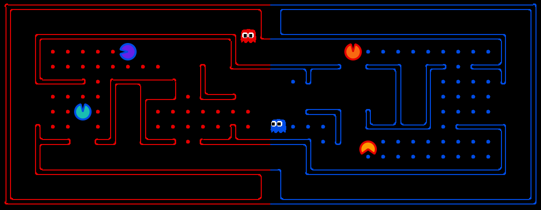
Overview
This contest involves a multiplayer capture-the-flag variant of Pacman, where agents control both Pacman and ghosts in coordinated team-based strategies. Each team will try to eat the food on the far side of the map, while defending the food on their home side. Students are expected to fuse the different AI tools acquired along this semester and produce a competitive, intelligent player.
Grading
Grading is assigned according to the following key:
- +1 points for over 51% winning rate against each of 3 staff bots
- +0.1 points per student bot beaten (>50% winning rate) in the final ranking
- 1st place: +2 points
- 2nd and 3rd place: +1.5 points
Introduction
The primary change between the first and this contests is that now it is an adversarial game, involving two teams competing against each other. Your team will try to eat the food on the far side of the map, while defending the food on your home side.
Your agents are in the form of ghosts on your home side and Pacman on your opponent's side. Also, you are now able to eat your opponent when you are a ghost. If Pacman is eaten by a ghost before reaching his own side of the board, he will explode into a cloud of food dots that will be deposited back onto the board.
Note that the contest framework, provided in contest3.zip,
has
changed slightly from Contest 1. The functions and interfaces are nearly the
same, but maps now include power capsules and you can eat your opponents.
External libraries: in this contest, you are allowed to use numpy as a dependency.
| Files you'll edit: | |
myTeam.py |
What will be submitted. Contains all of the code needed for your agent. |
| Files you might want to look at: | |
capture.py |
The main file that runs games locally. This file also describes the new capture the flag GameState type and rules. |
captureAgents.py |
Specification and helper methods for capture agents. |
baselineTeam.py |
Example code that defines two very basic reflex agents, to help you get started. |
| Supporting Files (Do not Modify): | |
game.py |
The logic behind how the Pacman world works. This file describes several supporting types like AgentState, Agent, Direction, and Grid. |
util.py |
Useful data structures for implementing search algorithms. |
distanceCalculator.py |
Computes shortest paths between all maze positions. |
graphicsDisplay.py |
Graphics for Pacman |
graphicsUtils.py |
Support for Pacman graphics |
textDisplay.py |
ASCII graphics for Pacman |
keyboardAgents.py |
Keyboard interfaces to control Pacman |
layout.py |
Code for reading layout files and storing their contents |
Files to Edit and Submit: You will fill and submit myTeam.py.
Academic Dishonesty: We will be checking your code against other submissions in the class for logical redundancy. If you copy someone else's code and submit it with minor changes, we will know. These cheat detectors are quite hard to fool, so please don't try. We trust you all to submit your own work only; please don't let us down. If you do, we will pursue the strongest consequences available to us.
Getting Help: You are not alone! If you find yourself stuck on something, contact the course staff for help. Office hours, section, and the discussion forum are there for your support; please use them. If you can't make our office hours, let us know and we will schedule more. We want these contests to be rewarding and instructional, not frustrating and demoralizing. But, we don't know when or how to help unless you ask.
Discussion: Please be careful not to post spoilers.
Rules
Layout
The Pacman map is now divided into two halves: blue (right) and red (left). Red agents (which all have even indices) must defend the red food while trying to eat the blue food. When on the red side, a red agent is a ghost. When crossing into enemy territory, the agent becomes a Pacman.
There are a variety of layout in the layouts directory.
Scoring
As a Pacman eats food dots, those food dots are stored up inside of that Pacman and removed from the board. When a Pacman returns to his side of the board, he "deposits" the food dots he is carrying, earning one point per food pellet delivered. Red team scores are positive, while Blue team scores are negative.
If Pacman gets eaten by a ghost before reaching his own side of the board, he will explode into a cloud of food dots that will be deposited back onto the board.
Power Capsules
If Pacman eats a power capsule, agents on the opposing team become "scared" for the next 40 moves, or until they are eaten and respawn, whichever comes sooner. Agents that are "scared" are susceptible while in the form of ghosts (i.e. while on their own team's side) to being eaten by Pacman. Specifically, if Pacman collides with a "scared" ghost, Pacman is unaffected and the ghost respawns at its starting position (no longer in the "scared" state).
Observations
Each agent can see the entire state of the game, such as food pellet locations, all pacman locations, all ghost locations, etc. See the GameState section for more details.
Winning
In this adversarial game, a team wins when they return all but two of the opponents' dots. Games are also limited to 1200 agent moves (moves can be unequally shared depending on different speeds - faster agents get more moves). If this move limit is reached, whichever team has returned the most food wins.
If the score is zero (i.e., tied) this is recorded as a tie game.
Computation Time
Each agent has 1 second to return each action. Each move
which does not return within one second will incur a warning. After
three warnings, or any single move taking more than 3 seconds, the game
is forfeit. There will be an initial start-up allowance of 15 seconds
(use the registerInitialState function).
Designing Agents
An agent now has the more complex job of trading off offense versus defense and effectively functioning as both a ghost and a Pacman in a team setting. The added time limit of computation introduces new challenges.
Baseline Team
To kickstart your agent design, we have provided you with a team of two baseline agents, defined in
baselineTeam.py. They are quite bad. The OffensiveReflexAgent simply moves
toward
the closest food on the opposing side. The DefensiveReflexAgent wanders around on its own
side
and tries to chase down invaders it happens to see.
File Format
You should include your agents in a file of the same format as myTeam.py. Your agents must
be
completely contained in this one file.
Interface
The GameState in capture.py should look familiar, but contains new methods like
getRedFood,
which gets a grid of food on the red side (note that the grid is the
size of the board, but is only true for cells on the red side with
food). Also, note that you can list a team's indices with getRedTeamIndices, or test
membership
with isOnRedTeam.
Distance Calculation
To facilitate agent development, we provide code in distanceCalculator.py to supply shortest
path maze distances.
CaptureAgent Methods
To get started designing your own agent, we recommend subclassing the CaptureAgent class.
This
provides access to several convenience methods. Some useful methods are:
def getFood(self, gameState):
Returns the food you're meant to eat. This is in the form of a matrix where
m[x][y]=True if there is food you can eat (based on your team) in that square.
def getFoodYouAreDefending(self, gameState):
Returns the food you're meant to protect (i.e., that your opponent is supposed to
eat). This is in the form of a matrix where m[x][y]=True if there is food at
(x,y) that your opponent can eat.
def getOpponents(self, gameState):
Returns agent indices of your opponents. This is the list of the numbers of the
agents (e.g., red might be [1,3]).
def getTeam(self, gameState):
Returns agent indices of your team. This is the list of the numbers of the agents
(e.g., blue might be [1,3]).
def getScore(self, gameState):
Returns how much you are beating the other team by in the form of a number that is the difference between your score and the opponents score. This number is negative if you're losing.
def getMazeDistance(self, pos1, pos2):
Returns the distance between two points; These are calculated using the provided
distancer object. If distancer.getMazeDistances() has been called, then maze distances are
available. Otherwise, this just returns Manhattan distance.
def getPreviousObservation(self):
Returns the GameState object corresponding to the last state this
agent
saw (the observed state of the game last time this agent moved).
def getCurrentObservation(self):
Returns the GameState object corresponding this agent's current
observation (the observed state of the game).
def debugDraw(self, cells, color, clear=False):
Draws a colored box on each of the cells you specify. If clear is
True,
will clear all old drawings before drawing on the specified cells. This
is useful for debugging the locations that your code works with. color:
list of RGB values between 0 and 1 (i.e. [1,0,0] for red) cells: list of game positions to
draw on (i.e. [(20,5), (3,22)])
Restrictions
You are free to design any agent you want. However, you will need to respect the provided APIs if you want to participate in the contest. Agents which compute during the opponent's turn will be disqualified. In particular, any form of multi-threading is disallowed, because we have found it very hard to ensure that no computation takes place on the opponent's turn.
Please respect the APIs and keep all of your implementation within myTeam.py.
Getting Started
By default, you can run a game with the simple baselineTeam that the staff has provided:
python capture.pyA wealth of options are available to you:
python capture.py --helpThere are four slots for agents, where agents 0 and 2 are
always on the red team, and 1 and 3 are on the blue team. Agents are
created by agent factories (one for Red, one for Blue). See the section
on designing agents for a description of the agents invoked above. The
only team that we provide is the baselineTeam. It is chosen by default as both the red and
blue
team, but as an example of how to choose teams:
python capture.py -r baselineTeam -b baselineTeamwhich specifies that the red team -r and the blue team -b are both created from
baselineTeam.py. To control one of the four agents with the keyboard, pass the appropriate
option:
python capture.py --keys0The arrow keys control your character, which will change from ghost to Pacman when crossing the center line.
Layouts
By default, all games are run on the defaultcapture layout. To test your agent on other
layouts, use the -l option. In particular, you can generate random layouts by specifying
RANDOM[seed]. For example, -l RANDOM13 will use a map randomly generated with
seed
13.
Recordings
You can record local games using the --record
option, which will write the game history to a file named by the time
the game was played. You can replay these histories using the --replay option and specifying
the file to replay.