Click on the image to see a PDF version (for zooming in)

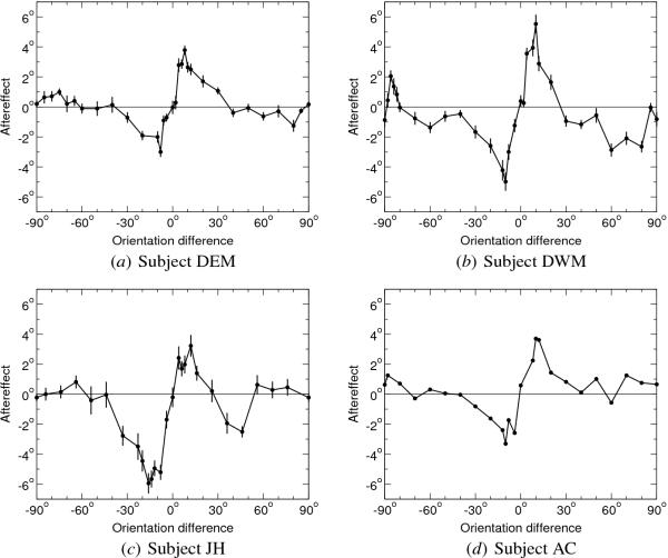
Fig. 7.2. Tilt aftereffect in human subjects. These plots show one TAE curve for each of the four subjects in Mitchell and Muir (1976): (a) DEM, (b) DWM, (c) JH, and (d) AC. The data were computed by averaging 10 trials before and 10 trials after adaptation. Error bars represent ±1 standard error of the mean (SEM); none were published for subject AC. Each trial consisted of a 3-minute adaptation to a sinusoidal grating, followed by a brief exposure to a test grating. The perceived orientation of the test grating was measured by having the subject adjust the orientation of a test line (presented in an unadapted portion of the visual field) until it appeared parallel to the test grating. For a given orientation difference counterclockwise between test and adaptation gratings, the TAE magnitude was then computed as the difference between the perceived orientations of the test grating before and after adaptation. In each case, a 0^o orientation difference represents the orientation of the adaptation grating. For DEM the adaptation grating was horizontal, for AC it was vertical, and for DWM and JH it was oblique (135^o). Similar direct effects were observed in all subjects, i.e. they perceived small orientation differences larger than they actually were; indirect effects varied more, but all subjects reported some contraction of large orientation differences.