Click on the image to see a PDF version (for zooming in)

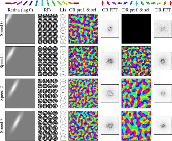
Fig. 5.25. Effect of input speed on direction maps. From left to right, each row shows a sample retinal activation at lag 0, final receptive fields to LGN regions with lags 3, 2, 1, and 0 (left to right) of six sample neurons, the inhibitory lateral connections of those six neurons, the orientation preference and selectivity map, the Fourier transform of the OR preferences, the direction preference and selectivity map, and the Fourier transform of the DR preferences. Orientation and direction histograms are not shown because they are all nearly flat. Each row shows the result from using training inputs moving at a different speed, ranging from zero (stationary) to moving three retinal units between each group of lagged LGN cells. For the example input shown, the lag 3 input was always the one shown in the top row (labeled "Speed 0"), and by lag 0 it had moved to the position shown in each row. When the inputs were stationary (i.e. all lags had the same input patterns), no direction map or directionselective units developed, and the "DR pref. & sel." map is entirely dark. As the speed increases, more units become direction selective, and direction becomes the largest-scale organization in the map. This increase in feature size is visible in the DR Fourier transform plots, where a smaller spatial frequency (larger feature spacing) leads to smaller rings as speed is increased. These results are predictions for maps in animals with different retinal motion sensitivities or those raised in environments with different speeds of visual motion.