Click on the image to see a PDF version (for zooming in)

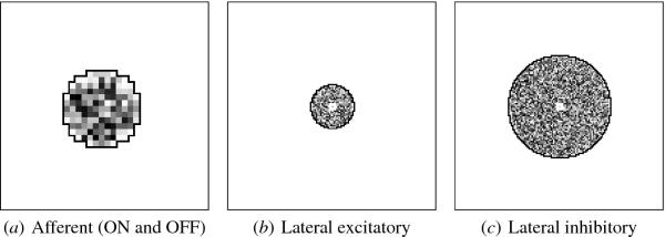
Fig. 4.3. Initial V1 afferent and lateral weights. The initial incoming weights of a sample neuron at the center of V1 are plotted in gray-scale coding from white to black (low to high). (a) The afferent RF center for each neuron was determined by first finding the location on the LGN that corresponds to the location of the neuron in V1, then randomly scattering the center by ±1.2 retinal units (5%) from that location. The neuron was then connected to LGN units within a radius of 6.5 from the center with random normalized weights. These weights are shown on the 36 × 36 LGN sheet, with the jagged black line tracing the RF boundary. The weights from the ON and OFF LGN sheets were initially identical. Plots (b) and (c) similarly show the lateral weights of this neuron, plotted on the 142 × 142 V1 and outlined with a black line. The neuron itself is marked with a small white square in the middle. The excitatory connections were initially random within a radius of 14.2, and inhibitory within 34.5 units. Later figures will show how these connections become organized through input-driven self-organization.