Click on the image to see a PDF version (for zooming in)

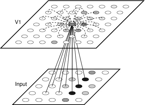
Fig. 3.3. General architecture of self-organizing map models of the primary visual cortex. The model typically consists of two sheets (also called layers, or surfaces) of neural units: input and V1. Some models also include a sheet of LGN neurons between the input and V1, or interpret the input sheet as the LGN; however, in most models the LGN is bypassed for simplicity, and the input sheet represents a receptor surface such as the retina. The input units are activated with continuous values according to the input pattern. In this example, the activations represent an elongated Gaussian, as shown in gray-scale coding from white to black (low to high). The input units are organized into a rectangular 5 × 5 grid; a hexagonal grid can also be used. Instead of grid input, some models provide the input features such as (x, y) position, orientation, or ocularity directly as activation values to the input units (Durbin and Mitchison 1990; Ritter et al. 1991). Others dispense with individual presentations of input stimuli altogether, abstracting them into functions that describe how they correlate with each other over time (Miller 1994). Neurons in the V1 sheet also form a two-dimensional surface organized as a rectangular or hexagonal grid, such as the 7 × 7 rectangular array shown. The V1 neurons have afferent (incoming) connections from neurons in their receptive field on the input sheet; sample afferent connections are shown as straight solid lines for a neuron at the center of V1. In some models the receptive field includes the entire input sheet (e.g. von der Malsburg 1973). In addition to the afferent input, the V1 neurons usually have short-range excitatory connections from their neighbors (shown as short dotted arcs) and long-range inhibitory connections (long dashed arcs). Most models save computation time and memory by assuming that the values of these lateral connections are fixed, isotropic, and the same for every neuron in V1. However, as will be shown in later chapters, specific modifiable connections are needed to understand several developmental and functional phenomena. Neurons generally compute their activation level as a scalar product of their weights and the activation of the units in their receptive fields; sample V1 activation levels are shown in gray scale. Weights that are modifiable are updated after an input is presented, using an unsupervised learning rule. In some models, only the most active unit and its neighbors are adapted; others adapt all active neurons. Over many presentations of input patterns, the afferent weights for each neuron learn to match particular features in the input, resulting in a map-like organization of input preferences over the network like those seen in the cortex.