Click on the image to see a PDF version (for zooming in)

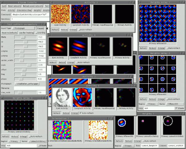
Fig. 17.3. Example Topographica screenshot. In this example session with Topographica, the user is studying the behavior of an orientation map in the primary visual cortex, using a model similar to the one depicted in Figure 17.2. The window at the bottom labeled "Orientation 1" shows the self-organized orientation map and the orientation selectivity in V1. The five windows labeled "Activity" show a sample visual image along with the responses of the retinal ganglion cells and V1 (labeled "Primary"; both the initial and the settled responses are shown). The input patterns were generated using the "Test pattern parameters" dialog at left. The window labeled "Weights 1" (lower right) shows the strengths of the connections to one neuron in V1. This neuron has afferent receptive fields in the ganglion cells and lateral receptive fields within V1. The afferent weights for 8 × 8 and 4 × 4 samplings of the V1 neurons are shown in the two "Weights Array" windows at right; most neurons are selective for Gabor-like patches of oriented lines. The inhibitory lateral connections for an 8 × 8 sampling of neurons are shown in the "Weights Array 3" window at lower left; neurons tend to receive connections from their immediate neighbors and from distant neurons of the same orientation. Topographica is designed to make this type of large-scale analysis of topographic maps practical, in addition to providing effective tools for constructing the models and their training and testing environments.