Click on the image to see a PDF version (for zooming in)

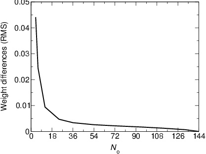
Fig. 15.8. Accuracy of the final GLISSOM map as a function of the initial network size. Each point shows the RMS difference between the final values of the corresponding weights of each neuron in two networks: a 144 × 144 LISSOM map, and a GLISSOM network with an initial size shown on the x-axis and a final size of 144 × 144. Both maps were trained on the same stream of oriented inputs. The GLISSOM maps starting at most as large as N = 96 were based on four scaling steps, whereas the three larger starting points included fewer steps: N = 114 had one step at iteration 6500, N = 132 had one step at iteration 1000, and there were no scaling steps for N = 144. Low values of RMS difference indicate that the corresponding neurons in each map developed very similar weight patterns. The RMS difference drops quickly as larger initial networks are employed, becoming negligible above 36 × 36. As was described in Section 15.2.3, this lower bound is determined by r_Ef, the minimum size of the excitatory radius.