Click on the image to see a PDF version (for zooming in)

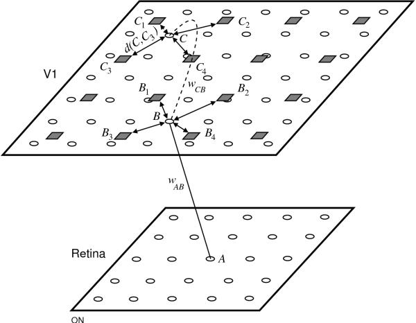
Fig. 15.5. Weight interpolation in GLISSOM. This example shows a V1 of size 4 × 4 being scaled to 7 × 7, with a fixed 8 × 8 retina. Both V1 networks are plotted in a continuous two-dimensional area representing the surface of the cortex. The squares in V1 represent neurons in the original network (i.e. before scaling) and circles represent neurons in the new, scaled network. A is a retinal receptor cell and B and C are neurons in the new network. Afferent connection strengths to neuron B in the new network are calculated based on the connection strengths of the ancestors of B, i.e. those neurons in the original network that surround the position of B (B₁, B₂, B₃, and B₄ in this case). The new afferent connection strength w_AB from receptor A to B is a normalized combination of the connection strengths w_ABi from A to each ancestor B_i of B, weighted inversely by the distance d(B, B_i) between B_i and B. Lateral connection strengths from C to B are calculated similarly, as a proximity-weighted combination of the connection strengths between the ancestors of those neurons. Thus, the connection strengths in the scaled network consist of proximity-weighted combinations of the connection strengths in the original network.