Click on the image to see a PDF version (for zooming in)

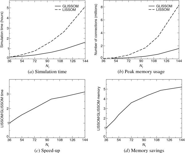
Fig. 15.10. Simulation time and memory usage in LISSOM vs. GLISSOM. Computational requirements of the two methods are shown as a function of the network size. In the LISSOM simulations the network had a fixed size N_f, as indicated on the x-axis; in GLISSOM the initial size was N_o = 36 and the final size N_f as indicated on the x-axis. Each point represents one simulation; the variance between multiple runs was negligible (less than 1% even with different input sequences and initial weights). (a) Simulation time includes training and all other computations such as plotting, orientation map measurement, and GLISSOM's scaling steps. The simulation times for LISSOM increase dramatically with larger networks, because larger networks have many more connections to process. In contrast, because GLISSOM includes fewer connections during most of the self-organizing process, its computation time increases only modestly for the same range of N_f. (b) Memory usage consist of the peak number of network connections required for the simulation; this peak determines the minimum physical memory needed when using an efficient sparse format for storing weights. LISSOM's memory usage increases very quickly as N_f is increased, whereas GLISSOM is able to keep the peak number low; much larger networks can be simulated on a given machine with GLISSOM than with LISSOM. (c,d) With larger final networks, GLISSOM results in greater speed-up and memory savings, measured as the ratio between LISSOM and GLISSOM simulation time and memory usage.