Click on the image to see a PDF version (for zooming in)

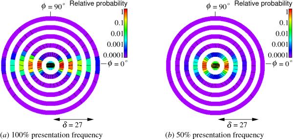
Fig. 13.21. Lateral excitatory connections in GMAP with different input frequencies. The connection probability distributions are displayed the same way as in Figure 13.9. As before, only GMAP is shown because it is responsible for contour integration in the model. The lateral connection profiles differ in two subtle ways: (1) The high probability areas (red and yellow) extend longer in the high-frequency map (a) than in the low-frequency map (b) (three vs. two rings of high probability). (2) The most probable &theta (black oriented bars) are cocircular in (a), but mostly collinear in (b) (as seen e.g. in the second ring from the outside). These results predict that contours should be easier to detect in the high-frequency network.