Click on the image to see a PDF version (for zooming in)

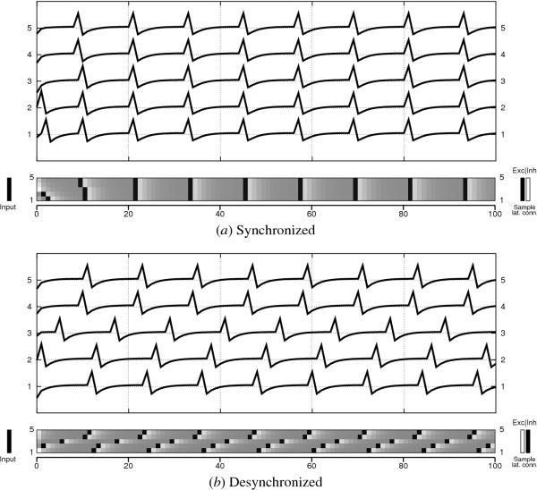
Fig. 12.1. Synchronized and desynchronized modes of firing. A network of five neurons is connected only with excitatory lateral connections in (a) and only with inhibitory lateral connections in (b), and exhibits synchronized and desynchronized firing as a result. Simulation time is shown on the x-axis, and the membrane potential for each neuron is displayed in two ways: along the y-axis in a voltage trace plot on the top, and in gray scale from white to black (low to high) in the bottom. Each row in each plot represents a different neuron, with its index identified on both sides of the plot (1 to 5, from bottom to top). The black vertical bar on the left shows which neurons are activated by afferent input (black means on and white means off); in these two examples, all input neurons were activated. To the right of the scatterplot, two vertical bars illustrate the excitatory (left) and inhibitory (right) lateral connection ranges of one sample neuron in the network; all neurons had identical connections in these two examples. Black indicates that a connection to the neuron exists in that row, and white that it does not. The same plotting convention will be used throughout this chapter. With excitatory lateral connections in (a), all spikes (peaks) start to become vertically aligned around iteration 21, showing that all the neurons are firing at the same time. In contrast, with inhibitory lateral connections in (b), the neurons all fire at different times. An animated demo of these examples can be seen at ...