Home

Assignment 3 (Part II) - Iterative Closest Point

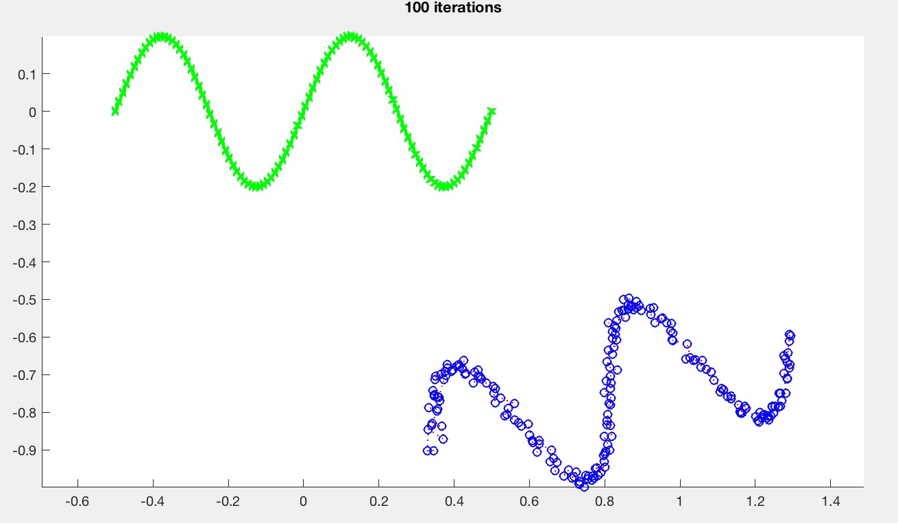
Due Monday 10/2 at 11:59 pm. You may work individually.

Overview

In this assignment, you are going to implement a simple version of the Iterative Closest Point algorithm in 2D.

Base Code

Start with the base Matlab code. Run the code by typing the following in the Matlab prompt:

>> driver(0)

The target curve is drawn in green, and the source curve is drawn in red. Since the base code does not yet implement ICP, the source curve is hidden behind the blue curve. Once ICP is implemented, the result should look something like this:

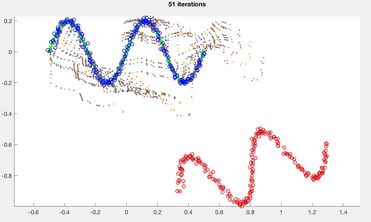
The small dots are the intermediate points during the search. You don't need to plot these in your implementation.

The driver creates the source and target curve points, which are both stored as 2xn matrices. So, to access the ith point in sourcePts, you need to specify that you want all the rows (specified by :) of the ith column:

sourcePts(:,i)

The resulting expression is a 2D column vector. To plot the points (see lines 33-37), say something like

plot(sourcePts(1,:),sourcePts(2,:),'r-');

which draws a red line with circles as markers and dotted lines connecting the markers. sourcePts(1,:) gets the 1st row of sourcePts, which corresponds to the X values of the source points. Again, the colon specifies that you want all the columns of the matrix. You can specify the line style by modifying the last arguments. Here, 'r-' draws a red line through the points.

The generatePts function generates the test data points. In a later task, you will be asked to add a new function in this file to generate more data.

The perturbPts function takes as input the data points and then adds random noise to the points, and then transforms (rotates and translates) the points. The goal of the ICP algorithm is to recover these rotation and translation parameters solely based on the perturbed source points and the target points.

The transformPts function takes the transformation parameters (stores as a 3D vector, see below) and transforms the points. Note that the actual transformation code is vectorized (line 9). The same thing can be accomplished by using a for-loop and iterating through all the points (source(:,i)), but Matlab runs much faster when you vectorize your code. For this assignment, do not worry about vectorizing. It is more important to have clean, readable code.

Task 1

The pseudocode for ICP is as follows:

1. Select e.g. 1000 random sample points from the source.
2. Match each sample to the closest point on the target.
3. Reject pairs with distance > k times the median distance.
4. Optimize for the best \theta, x, y to be applied to the source so that the pair distances are minimized.

The steps above are repeated until convergence or until the maximum number of iterations is reached.

For this task, ignore steps 1 and 3. Since I have already written the necessary function for step 4, the only things that need to be done are step 2 and the convergence check. Take a look again at icp2d.m. This function takes as input the source and target points, and computes as output the appropriate values of \theta, x, y. The main iteration loop is at the end of the function:

% Current theta, x, and y, stored as a column vector:
% thetaXY(1) is theta
% thetaXY(2) is x
% thetaXY(3) is y
thetaXY = [0 0 0]';
for iter = 1 : iterMax
    % Do something here
end

For this task, the ICP steps 2 and 4 need to go inside this loop.

The very first thing inside the loop should be to compute the new transformed points using the current values of \theta, x, y. To do this, add the following inside the loop:

sourcePts1 = transformPts(thetaXY,sourcePts);

Set iterMax in driver.m to 1 for now. Try hard-coding various values for \theta, x, y by modifying the thetaXY variable and plotting the resulting transformed points. The goal of the ICP algorithm is to find these values automatically.

To complete step 2, you need to first understand what is required for step 4, which is outlined below.

For step 4, we are going to use Matlab's powerful fminunc optimization function. I have already written the objective function (distFun), so the only thing you need to do is to call

thetaXY1 = fminunc(@(thetaXY)distFun(thetaXY,sourcePts,targetPts,closest),thetaXY,opt);

The output, thetaXY1, is the (locally) optimal \theta, x, y computed by fminunc. The second-to-last argument, thetaXY, is the initial guess for fminunc, for speeding up the search. You should use the \theta, x, y values from the previous iteration as this initial guess.

The closest argument stores which target points are closest to each of the source points. This needs to be computed in the matching step.

• The length of the closest vector should be number of points in the source.
• The ith element of closest stores the index of the closest target point from the ith source point.

For example if closest = [4 5 4 2 ...], then the first source point's closest point is targetPts(:,4), the second source point's closest point is targetPts(:,5), and so on.

To test for convergence, check whether the newly computed values of \theta, x, y are close to the previous values of \theta, x, y. A simple L2 norm will suffice. I.e., check if \sqrt{\Delta \theta^2 + \Delta x^2 + \Delta y^2} is less than thresh.

If the initial guess is too far, then ICP may not converge to a good local minimum. Modify the random perturbation factors (lines 14-17 in driver.m) until you get something that behaves well.

theta = randBetween(-30.0,30.0)*pi/180.0;
x = randBetween(-1.0,1.0);
y = randBetween(-1.0,1.0);
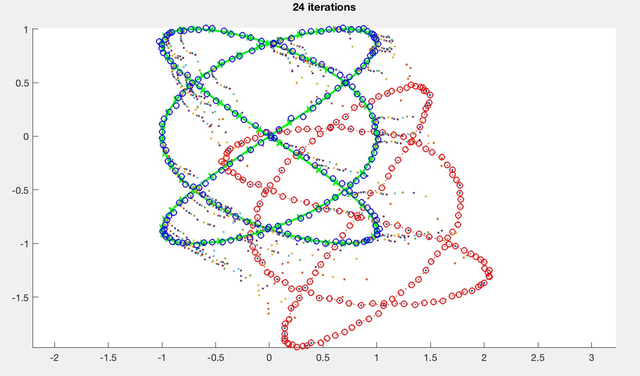
noise = 0.01;

Task 2

The argument to the driver function controls the generated curves. driver(0) produces sine curves, and driver(1) produces Lissajous curves. Here is the matched Lissajous curves after ICP is implemented.

Create at least one more curve type in generatePts.

Task 3

Implement steps 1 and 3 from the pseudocode above.

Step 1 makes ICP scalable, which is especially important for 3D surfaces. Since we're doing 2D curves, the speed might not change much for us here.

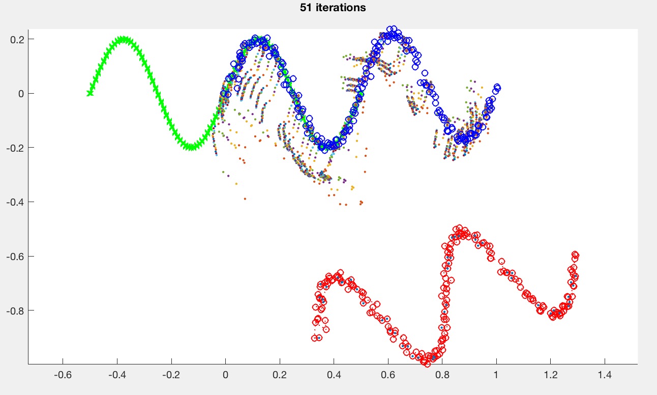
Step 3 allows ICP to get partial matches. Use the medianMult argument as the k in the pseudocode above. medianMult=inf implies that no pairs will be rejected, which means that the behavior should default back to the previous version from Task 1. This value depends on the type of the curve. For the sine curve (caseNumber=0), with medianMult=2, you should be able to get something like this:

Evaluation

• For a grade of B, you must finish Tasks 1 and 2, and submit a report (see below).
• For a grade of A, you must also finish Task 3.

What to hand in

Please provide a report with your submission (PDF). The report should include the following:

• Your name
• For each of the figures, provide the parameters (e.g., noise, thresh, iterMax, etc.) for reproducing the figure.
• Figures from the sine curve, Lissajous curve, and at least one more curve of your own design.
• For each curve above, show one case where ICP worked and one case where it didn't work. Explain why ICP didn't work.
• If you did Task 3, show a partial match as in the figure above. What happens when medianMult is too big or too small? What happens if the number of samples is too small?
• Do you have any comments about this assignment that you would like to share?

Create a zip file named NETID.zip (your email ID; e.g., sueda.zip) so that when you extract it, it creates a folder called NETID/ (e.g., sueda/) that has (ONLY) the following in it:

• Your PDF report
• Your Matlab files