In this lab, we’re going to create pretty graphics with a particle system.
Please download the lab and go over the code.
We are using a C++ library called Eigen. You’ll have to install this in the same way you installed glm in lab 0. You’ll need to create a new environment variable called EIGEN3_INCLUDE_DIR that points to the Eigen directory. Once you have it installed, you may want to look at this quick tutorial.
OPTIONAL READING: Note the following techniques I am using to draw the particles.
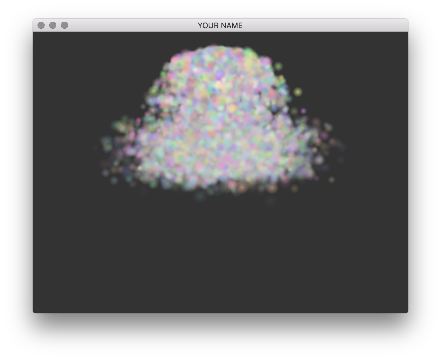
GL_POINTS. These points are drawn as “billboarded” quads. To control the size of each quad that gets generated from each point, I am writing to a special output called gl_PointSize in the vertex shader. This feature, GL_PROGRAM_POINT_SIZE is enabled in main.cpp. See http://stackoverflow.com/questions/17397724/point-sprites-for-particle-system and http://stackoverflow.com/questions/25780145/gl-pointsize-corresponding-to-world-space-size for more information.alpha.jpg. For each “billboarded” quad, the texture coordinates of the fragments are automatically computed by OpenGL and stored in a special varying attribute called gl_PointCoord. Then, any texture can be applied to GL_POINTS. The classic approach to enable alpha blending requires sorting the particles from back to front, but here I am using another approach that does not require sorting. See http://gamedev.stackexchange.com/questions/9436/order-independent-transparency-in-particle-system/24489 for more information.Vector3f, then copying this data one by one into an OpenGL buffer would be very wasteful. Instead, I store the particle position as a Eigen::Map<Eigen::Vector3f>, which allows me to define an Eigen::Vector3f that is mapped to a specific location in a vector<float>. This allows me to directly update the 3 floats in the buffer. See http://eigen.tuxfamily.org/dox/group__TutorialMapClass.html for more information.Run the code: press the space bar and watch a never-ending sequence of explosions. This is a 3D explosion — you can rotate the scene with the mouse as before. Also, try increasing the number of particles by modifying init(). On my laptop, I can easily go up to 10,000 particles.
Change the Particle::rebirth(...) function so that more things are randomized appropriately. Use the randFloat(low, high) function to choose some values you like. Play around with some values to get an intuition on what these parameters do.
x (initial position): Where the particle starts from.v (initial velocity): How fast and in which direction the particle is moving initially.d (viscous damping): How quickly the particles lose energy (implemented later).lifespan: How many seconds each particle lives. Once a particle dies, its rebirth() function is called.You may also change the color and the size of the particles by modifying the constructor.
Currently, each particle moves in a straight because the physics has not been fully implemented. Modify Particle::step() to do the following:
Accumulate force: First, we’ll only have the force of gravity. Create a \(3 \times 1\) vector f and set it to be the force of gravity using the gravity vector passed into the function from main.cpp: \[
\vec{f} = m \vec{g},
\] where \(m\) is the mass of the particle. We’ll add more forces later in this lab.
Integrate velocity: \[ \vec{v}_{\text{new}} = \vec{v}_{\text{old}} + \frac{h}{m} \vec{f}. \]
Integrate position: \[ \vec{x}_{\text{new}} = \vec{x}_{\text{old}} + h \vec{v}_{\text{new}}. \] This line is already implemented for you.
This scheme is called Symplectic Euler integration. Keep in mind that x, v, and f are all \(3 \times 1\) vectors.
You should try running your code in release mode (See lab 0) so that you can simulate more particles.
We can easily add other types of forces by changing Step 1 from the previous task. First, add viscous damping force:
\[ \vec{f} = −d \vec{v}, \]
where \(d\) is the viscous damping coefficient. (This force does not replace the force of gravity. You should add them up since we want both.) This applies a negative force proportional to the velocity of the particle. Try changing d to see what values look good. Don’t make this value too large, or else you’ll run into numerical problems.
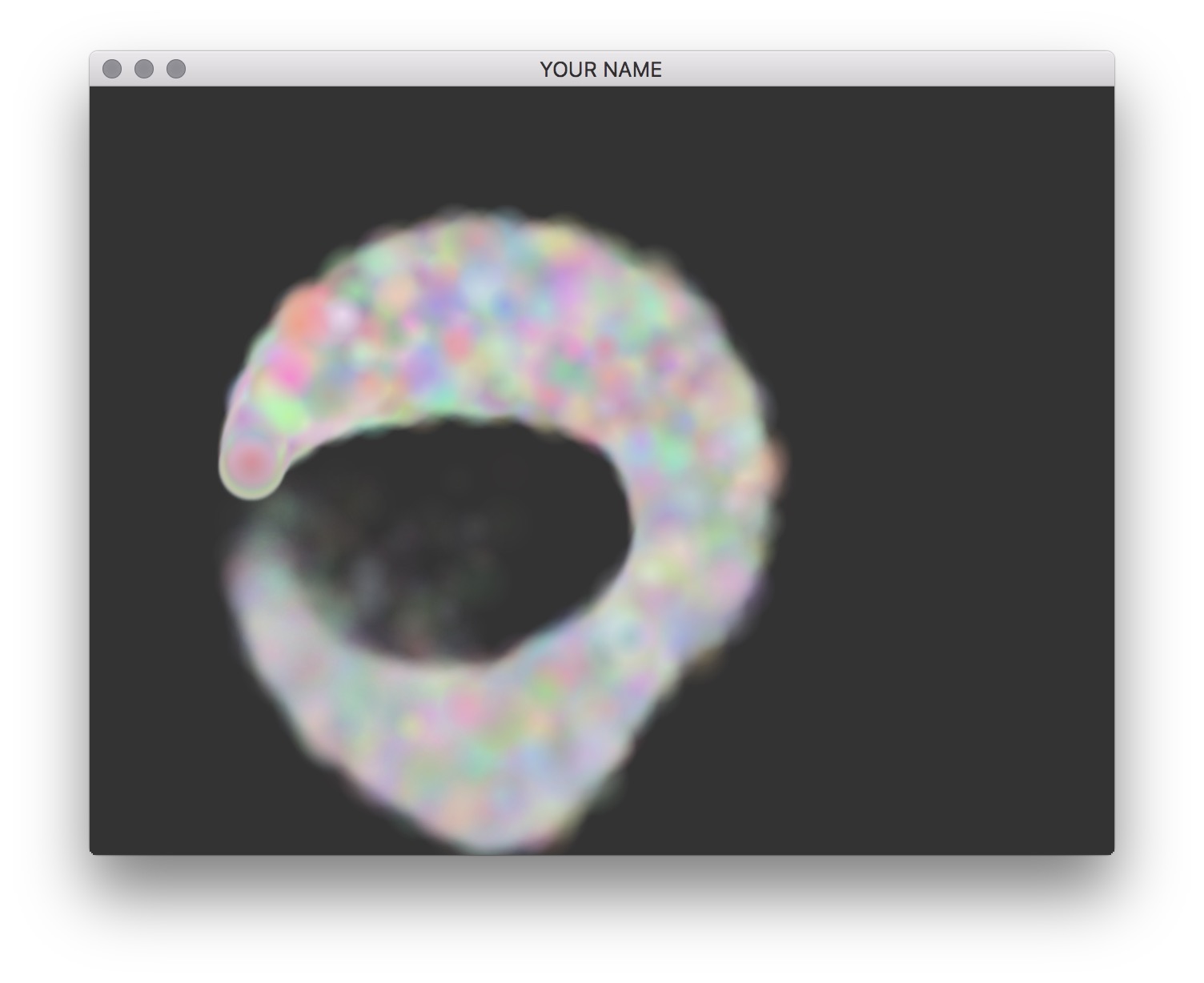
The force of gravity we have implemented so far assumes that the force of direction is constant everywhere. (This is the assumption we usually make on the earth’s surface.) Now we’ll add another type of gravity that is more general. Use keyToggles[’g’] to toggle between these two types of gravity. The new gravity force follows the inverse square law. The force magnitude falls off as the inverse square of the distance. We’ll use the world origin to measure the distance. We’ll use the softened version of the force, which was developed by astrophysicists so that division by \(0\) does not occur when the orbital distance becomes too small.
\[ \vec{f} = -\frac{C m}{\left( \| \vec{x} \|^2 + \varepsilon^2 \right)^\frac{3}{2}} \vec{x}, \]
where \(C\) is a constant you choose, \(m\) is the mass of the particle, \(\vec{x}\) is the position of the particle, and \(\varepsilon^2\) is the “softening length,” which you should set to a small number, such as 0.01f. Play with \(C\) and \(\varepsilon^2\) to get a sense of what they do.
Add collision with the floor (the \(y=0\) plane) to the end of Particle::step(). If you detect that the particle is below the floor, set its position to be at the floor and flip its velocity with respect to the floor. The particle’s tangential velocity should remain fixed, while its normal velocity should be flipped. Add a toggle for this with the f key.