Due Wednesday, 11/10 at 23:59:59. You must work individually.
In this assignment, we’re going to simulate cloth with linearly implicit Euler, penalty collision forces, and sparse matrices.
Please download the assignment and go over the code.
Your main task is to complete the function Cloth::step(). I have written a lot of code for you that deal with setting up the scene and rendering the cloth. Study the code carefully to see what is happening.
main()
h key runs one simulation step.Scene
This class is responsible for holding the things in the scene. Currently it holds a pointer to a cloth, and an empty vector of pointers to spheres.
To change the number of rows and columns of the cloth, modify Scene::load(). You should start with a 2 by 2 cloth.
Particle
The particle class is used to represent both cloth nodes and spheres.
It has position x and velocity v.
The radius r is used for collisions. A cloth particle has a small radius that is noticeably larger than the thickness of the cloth.
Cloth
Cloth::Cloth()
The particles and the springs are created. The particles are created from a grid with corners x00, x01, x10, and x11. There are ‘x’ springs, ‘y’ springs, two sets of ‘shear’ (or diagonal) springs, and two sets of ‘bending’ springs.
Each particle knows its starting index into the global vectors and matrices (lines 64 and 67). For example, if the starting index of a particle is 3, then the particle’s indices are {3,4,5}. If a particle is fixed to the world, it gets the index of -1.
The global matrices and vectors are allocated (line 121).
The vertex buffers for rendering the cloth are allocated (line 127).
Cloth::updatePosNor()
Cloth::draw()
At each time step, you must fill in \(M, K, v\), and \(f\) with appropriate values, and then solve the linear system
\[ A x = b, \]
where
\[ \begin{aligned} A &= M - h^2 K\\ b &= M v + h f. \end{aligned} \]
The solution, \(x\), of the linear system contains the new velocities of the particles.
For solving a linear system, we are using a C++ library called Eigen. You’ll have to install this in the same way you installed glm in lab 0. You’ll need to create a new environment variable called EIGEN3_INCLUDE_DIR that points to the Eigen directory. Once you have it installed, you may want to look at this quick tutorial.
We’ll start with symplectic Euler, which boils down to the same thing as above but with \(A=M\), which means you don’t need to form \(K\) yet.
In Cloth::Step(), loop through the particles to fill in \(M\) and \(v\), and fill in \(f\) with gravity. (Note the const Vector3d &grav argument of Cloth::step().) Use the block() and segment() functions in Eigen. Remember to not fill in these values for fixed particles. (I.e., only add these values for free particles.) The indices of the particles are stored inside the particle class Particle::i. This is the starting index of the particle into \(M,\) \(v,\) and \(f\). For example, if the index of a particle is 6, then you should store its velocity into the \(v\) vector at indices 6, 7, and 8.
In the same function, loop through the springs to add spring forces to \(f\). Remember to add to \(f\), rather than setting the values of \(f\). (In other words, we want += rather than =.) Each spring object contains pointers to the two particles attached to the spring. The formula for the spring force is
\[ \begin{aligned} & f_s = E (l-L) \frac{\Delta x}{l},\\ & f = \begin{pmatrix} f_s \\ -f_s \end{pmatrix}, \end{aligned} \]
where \(E\) is the stiffness constant, \(\Delta x = x_1 − x_0\) is the vector between the two particle positions, \(l = \| \Delta x \|\) is the current spring length, and \(L\) is the spring’s rest length. (Each spring is between particle 0 and particle 1.) This force, \(f_s\), is the force for particle p0 of the spring. The force for the other particle p1 is the negation, \(-f_s\). Again, remember to add this force only to free particles.
Solve the linear system \(A x = b\). There are many linear solvers provided by Eigen. The LDLT solver is a good choice for now: A.ldlt().solve(b). The resulting solution \(x\) contains the new velocities of the particles.
Loop through the particles to extract the velocities from the solution vector.
Loop through the particles one last time to integrate the positions using the new velocities.
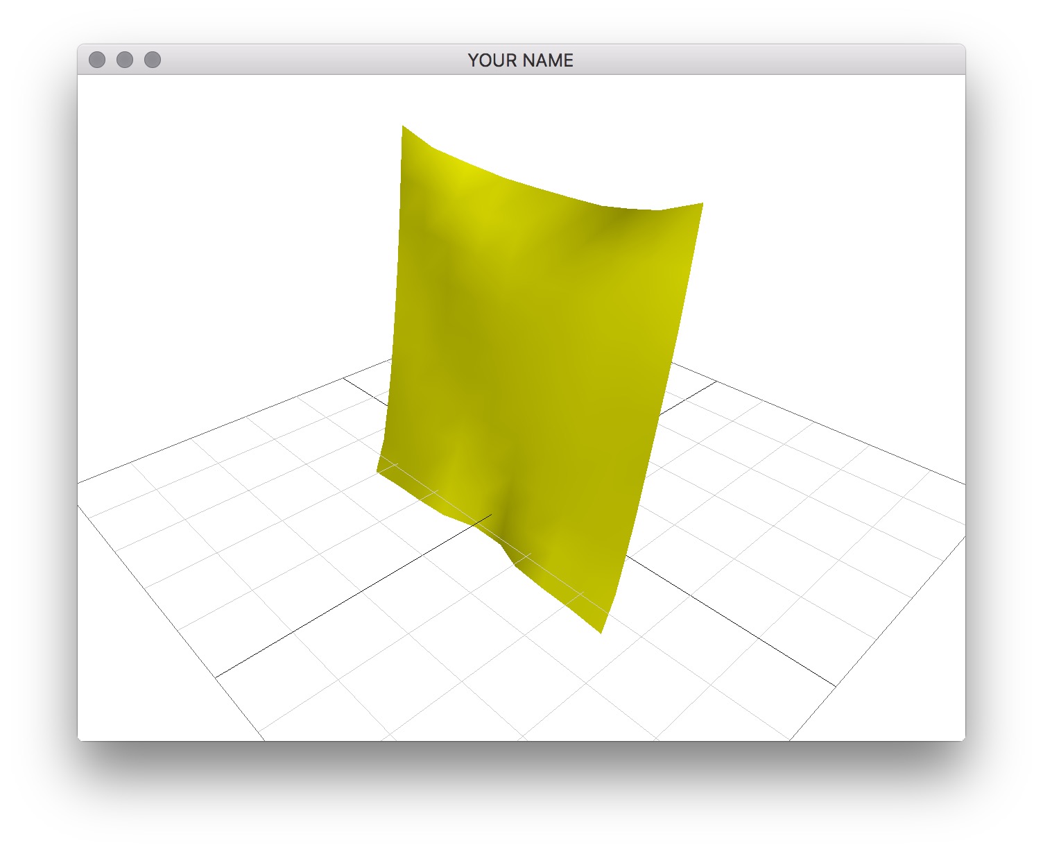
With symplectic Euler, you should be able to simulate a \(2 \times 2\) system with h=5e-3 and stiffness=1e1. You should see a cloth that looks like a flat sheet that does not bend. Try changing these values - you’ll see that the simulation quickly becomes unstable. One of the best ways to make it stable is to implement implicit integration, which is our next task.
Now implement implicit Euler by filling in and using the stiffness matrix, \(K\). The formula for the \(2 \times 2\) block stiffness matrix for a spring is
\[ \begin{aligned} & K_s = \frac{E}{l^2} \left( \left(1 - \frac{l-L}{l} \right) \left( \Delta x \Delta x^T \right) + \frac{l-L}{l} \left( \Delta x^T \Delta x \right) I \right),\\ & K = \begin{pmatrix} -K_s & K_s \\ K_s & -K_s \end{pmatrix}. \end{aligned} \]
Note that \(\Delta x^T \Delta x\) is a scalar, and \(\Delta x \Delta x^T\) is a \(3 \times 3\) matrix. \(I\) is the \(3 \times 3\) identity matrix.
This \(2 \times 2\) block matrix, \(K\), should be added to the global stiffness matrix into the appropriate rows/cols using the indices of the two particles. Again, remember to not add these values for fixed particles. The off-diagonal values should be added only if both particles of the spring are free.
With the following settings in Scene::Scene():
h = 5e-3;
grav << 0.0, -9.8, 0.0;
int rows = 2;
int cols = 2;
double mass = 0.1;          // total mass of the cloth
double stiffness = 1e1;     // E
the \(A\) matrix and the \(b\) vector should be the following for the very first step.
cout << A << endl;
    0.0254         0    0.0001   -0.0003         0         0
         0    0.0250         0         0         0         0
    0.0001         0    0.0254         0         0         0
   -0.0003         0         0    0.0254         0   -0.0001
         0         0         0         0    0.0250         0
         0         0         0   -0.0001         0    0.0254

cout << b << endl;
         0
   -0.0012
         0
         0
   -0.0012
         0
A common bug is that the sign of the stiffness matrix \(K_s\) is flipped. Try negating it!
Try increasing the cloth resolution to \(10 \times 10\) or higher. You may have to play around with the time step and stiffness values to make the cloth stable.
You should try running your code in release mode (See lab 0) so that you can simulate more particles.
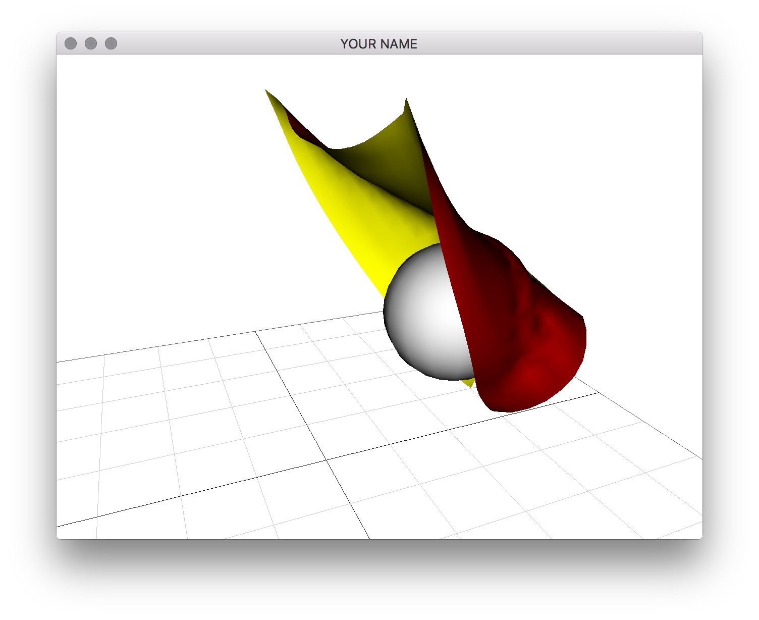
If you uncomment line 91 in Scene::draw(), you’ll see a collision sphere moving, but it won’t be affecting the cloth yet. We need to write some collision code first.
Implement collisions in Cloth::step(), right before the linear solve. You must check all the cloth particles against all the collision spheres (which are also particles) in the scene, which in this case is just a single sphere. For each particle, if there is a collision, add a collision force to the RHS and the corresponding implicit term to the LHS. Unlike cloth spring forces, these collision forces act on a single particle.
To compute the collision normal, we use the positions of the particles and the sphere. Let \(\vec{x}\) be the position of the particle, and \(\vec{x}_s\) be the position of the sphere. Then the vector from the sphere to the particle is \(\Delta\vec{x} = \vec{x} - \vec{x}_s\). Let \(l = \| \Delta\vec{x} \|\) be the length of \(\Delta x.\) The collision normal is then \(\vec{n} = \frac{\Delta\vec{x}}{l}\). To obtain the penetration depth, we subtract \(l\) from the sum of the radii of the sphere and the particle: \(d = r + r_s - l\). If this distance, \(d,\) is positive, then we have detected a collision. The collision force is computed using the depth and the normal:
\[ f_c = c d \vec{n}, \]
where \(c\) is the collision stiffness constant. The stiffness matrix entry can be approximated simply as:
\[ K_c = c d I, \]
where \(I\) is the \(3 \times 3\) identity matrix.
If you’re planning to use cloth simulation for your project, I highly recommend converting your code to use sparse matrices instead of dense matrices. On my computer, for a \(30 \times 30\) cloth, sparse is noticeably faster than dense. For a bigger system, the difference will be extremely significant. See Eigen’s sparse matrix tutorial.
You have to modify your matrix filling code and matrix solving code. To fill a sparse matrix, you must first create an array of triplets of the form row, col, val. As an example, the code to create a sparse \(2 \times 2\) identity matrix is
typedef Eigen::Triplet<double> T;
std::vector<T> A_;
A_.push_back(T(0, 0, 1));
A_.push_back(T(1, 1, 1));
Eigen::SparseMatrix<double> A(2,2);
A.setFromTriplets(A_.begin(), A_.end());
Not everything needs to be sparsified.
To solve using a sparse matrix, we must use a specialized sparse solver. There are many options, but for animation purposes, running Conjugate Gradients (CG) for several iterations is often sufficient. The following code solves \(A\vec{x} = \vec{b}\) with CG.
ConjugateGradient< SparseMatrix<double> > cg;
cg.setMaxIterations(25);
cg.setTolerance(1e-6);
cg.compute(A);
VectorXd x = cg.solveWithGuess(b, x0);
For CG, it is important to give the initial guess, x0. In our case, x represents the new particle velocities, so you should use the previous particle velocities as the initial guess.
With sparse matrices implemented, try increasing the resolution to \(30 \times 30\).
Total: 100 points
Failing to follow these points may decrease your “general execution” score.
If you’re using Mac/Linux, make sure that your code compiles and runs by typing:
> mkdir build
> cd build
> cmake ..
> make
> ./A5 <SHADER DIR>
If you’re using Windows, make sure your code builds using the steps described in Lab 0.
(*.~), or object files (*.o). You should hand in the minimum set of files you need to compile plus the README file.USERNAME.zip (e.g., sueda.zip). The zip file should extract everything into a folder named USERNAME/ (e.g. sueda/).
src/, resources/, CMakeLists.txt, and your README file to the USERNAME/ directory..zip format (not .gz, .7z, .rar, etc.).