Today we’re going to minimize a scalar function of two variables using:
Please download the code for the lab and go over the code. This lab uses Eigen for linear algebra. Although we could use GLM because our minimization variable is only 2D, we’re going to use Eigen so that you can use your code later for future projects. You’ll have to install Eigen in the same way you installed GLM in lab 0. You’ll need to create a new environment variable called EIGEN3_INCLUDE_DIR that points to the Eigen directory. Once you have it installed, you may want to look at this quick tutorial.
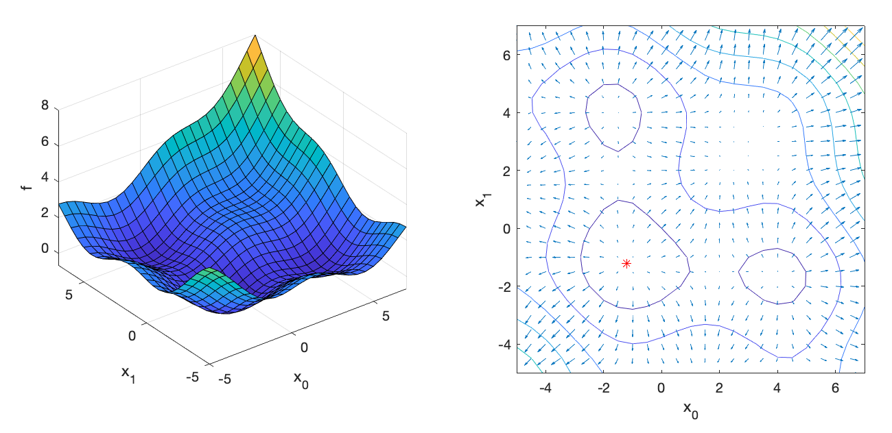
The objective function we’re going to minimize is:
\[ \displaylines{ f(\vec{x}) = \frac{1}{2} \sin(x_0) + \frac{1}{2} \sin(x_1) + \frac{1}{20} x_0^2 + \frac{1}{20} x_0 x_1 + \frac{1}{20} x_1^2 \\ \vec{g}(\vec{x}) = \begin{pmatrix} \frac{1}{2} \cos(x_0) + \frac{1}{10} x_0 + \frac{1}{20} x_1\\ \frac{1}{2} \cos(x_1) + \frac{1}{20} x_0 + \frac{1}{10} x_1 \end{pmatrix}\\ H(\vec{x}) = \begin{pmatrix} -\frac{1}{2} \sin(x_0) + \frac{1}{10} & \frac{1}{20}\\ \frac{1}{20} & -\frac{1}{2} \sin(x_1) + \frac{1}{10} \end{pmatrix}. } \]
The minimum is at [-1.201913 -1.201913].
There are three eval() methods in the class ObjectiveL06. The first one returns just the objective value, the second one returns the objective and the gradient, and the third one returns the objective, gradient, and the Hessian. Fill these methods to compute the expression given above. If implemented properly, with the input argument x = [4.0, 7.0], the returned values should be:
f = 4.6001;
g = [
    0.4232
    1.2770
    ];
H = [
    0.4784    0.0500
    0.0500   -0.2285
];Implement the following pseudocode in OptimizerGD.cpp:
for iter = 1 : iterMax
    Evaluate f and g at x
    dx = -alpha*g
    x += dx
    if norm(dx) < tol
        break
    end
end
If implemented properly, the optimizer should converge after 82 iterations to x = [3.294, 3.294]:
=== Gradient Descent ===
x = [
3.29446
3.29447];
82 iterations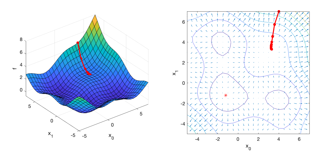
Implement the following pseudocode in OptimizerGDLS.cpp:
for iter = 1 : iterMax
    Evaluate f and g at x
    % Line search
    alpha = alphaInit
    while true
        dx = -alpha*g
        Evaluate fnew at x + dx
        if fnew < f
            break
        end
        alpha *= gamma;
    end
    x += dx
    if norm(dx) < tol
        break
    end
end
If implemented properly, the optimizer should converge after 27 iterations to x = [-1.202, -1.202]:
=== Gradient Descent with Line Search ===
x = [
-1.20191
-1.20191];
27 iterations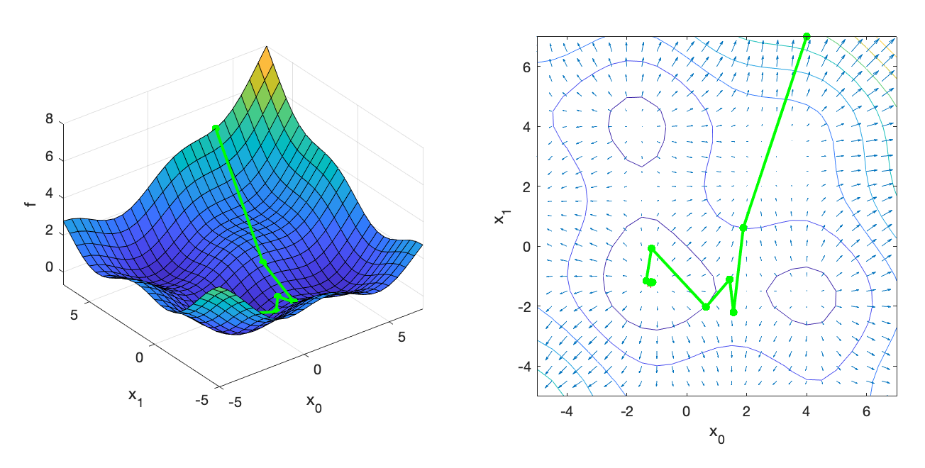
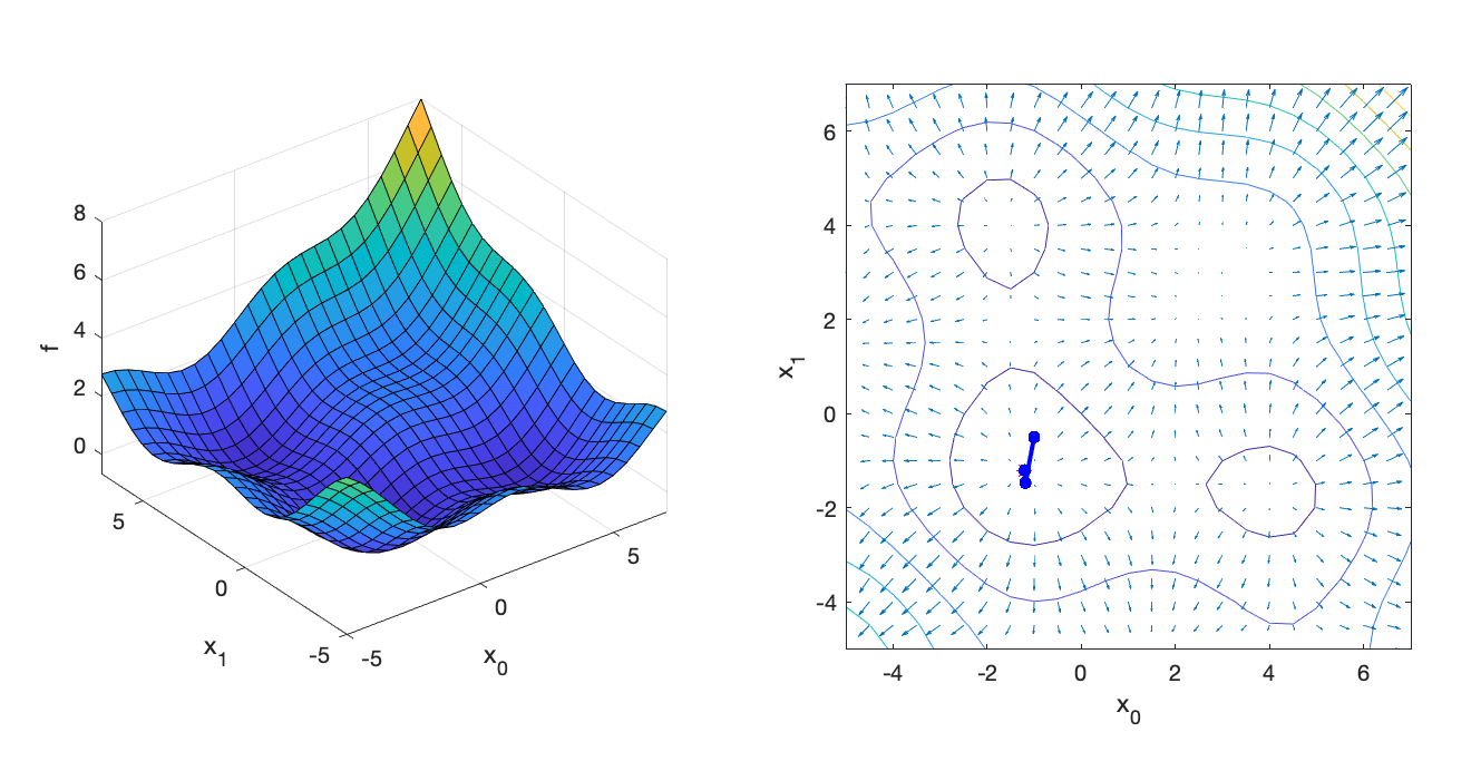
Implement the following pseudocode in OptimizerNM.cpp:
for iter = 1 : iterMax
    Evaluate f, g, and H at x
    dx = -H\g
    x += dx
    if norm(dx) < tol
        break
    end
end
The notation x = A\b is the MATLAB notation for solving the linear system \(Ax=b\). It is important to use an appropriate numerical solver for this operation. (Do not use the inverse!) Assuming that Hessian is symmetric positive definite (nice and convex), we can use Eigen’s LDLT solver: x = A.ldlt().solve(b). If implemented properly, the optimizer should converge after 9 iterations to x = [3.294, 3.294]:
=== Newton's Method ===
x = [
3.29446
3.29446];
9 iterations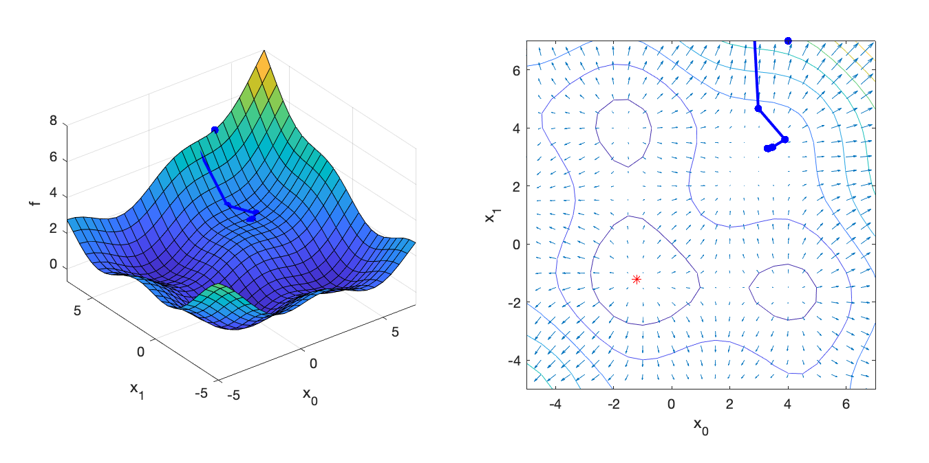
If we start the search at xInit = [-1.0, -0.5] instead, Newton’s Method converges to the minimum quickly:
=== Newton's Method ===
x = [
-1.20191
-1.20191];
5 iterations