In this lab, we’re going to use arc length parameterization to draw equally spaced points on a cubic spline curve.
Please download the lab and go over the code.
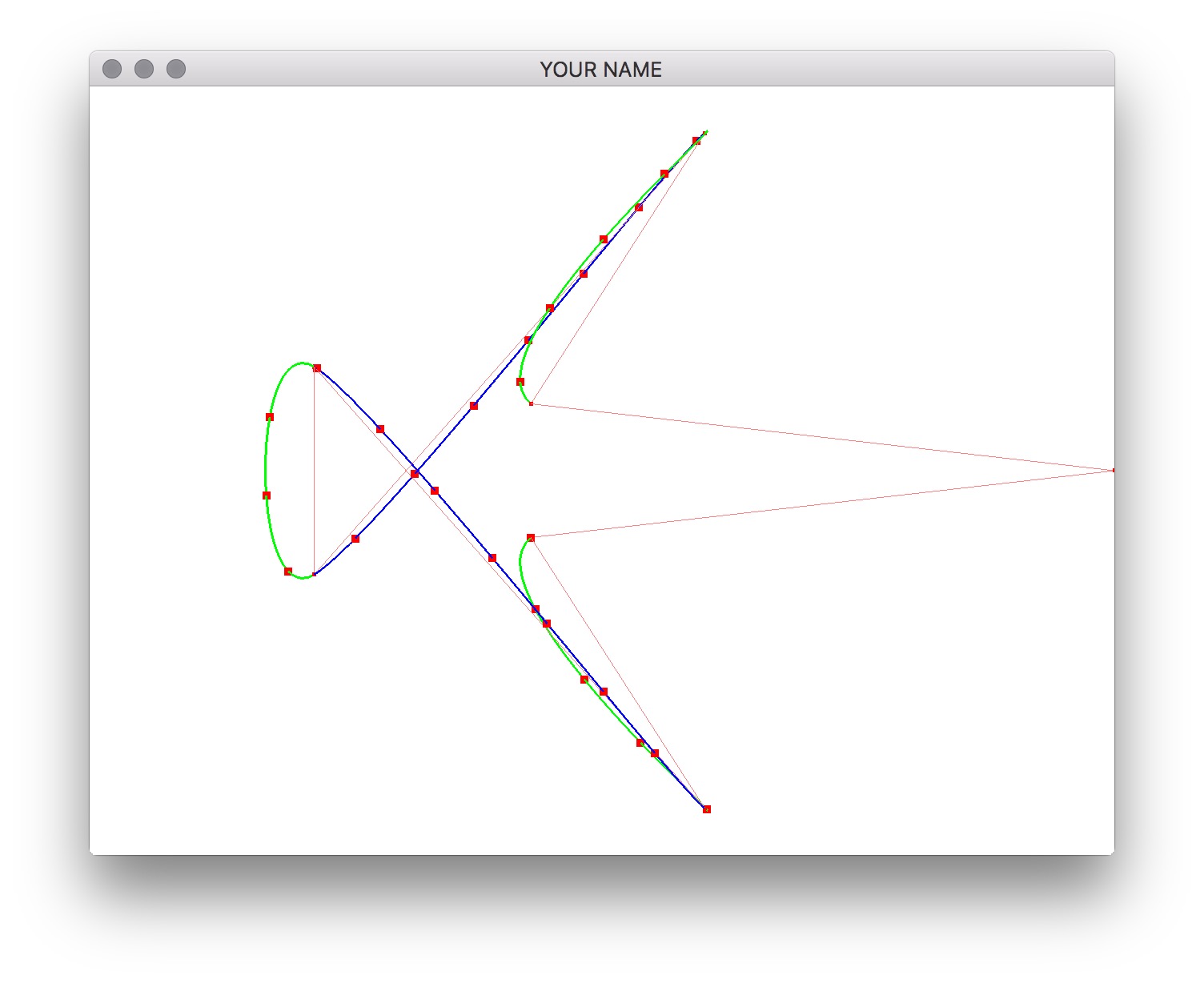
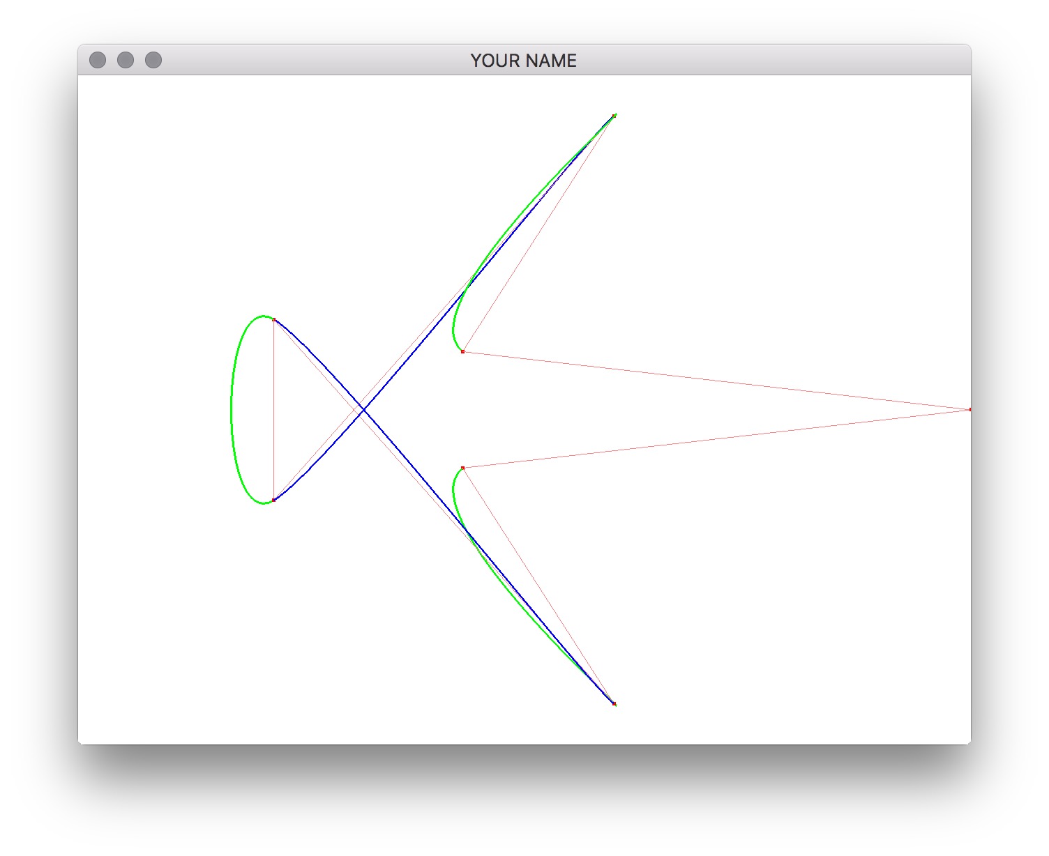
When you compile and run the source code, you should be able to insert control points by shift clicking, and rotate the camera by clicking and dragging the mouse. Press the r key to load some preset control points, and the c key to clear. We’re going to use this scene as the test case, so do not change this part of the code. The curve is now colored in green and blue. Each color corresponds to a segment defined by four control points.
There are two functions to implement: buildTable() and s2u(). (Feel free to add other functions though!) Note that the spline basis matrix, B, is constructed using the line:
glm::mat4 B = (type == CATMULL_ROM ? Bcr : Bb);The contents of Bcr and Bb are already defined for you.
First, write the function, buildTable(), which builds the table that lists the s value for each u. Here, s is the total distance traveled along the curve, and u is the concatenated spline parameter in the range [0, ncps-3]. (ncps is the number of control points.) There is a global variable called usTable that stores this information as an STL vector. The class type of this variable is std::vector<std::pair<float,float> >. (Note that when defining nested template types, you should insert a space between the closing brackets: > >.) To add a new row to this table (i.e., new element to this vector), use the push_back() and the make_pair() function calls. For example, the very first row should be [u=0, s=0], so you should call usTable.push_back(make_pair(0.0f, 0.0f));.
Use 5 samples for each segment to compute the distance along the curve. Since there are 8 control points in the preset test scene (press r), there are \(8-3=5\) segments. This means that \(u\) should take on the values \(0.0, 0.2, 0.4, \cdots, 4.8, 5.0\). First, use the simple formula to compute the distance between two u values, \(u_A\) and \(u_B\).
\[ \begin{aligned} \bar{P}(u_A) &= G B \bar{u}_A,\\ \bar{P}(u_B) &= G B \bar{u}_B,\\ s &= \| \bar{P}(u_B) - \bar{P}(u_A) \|. \end{aligned} \]
The values should look like this for the preset test scene with Catmull-Rom.
| u | s |
|---|---|
| 0.0 | 0.00000 |
| 0.2 | 0.13984 |
| 0.4 | 0.35787 |
| 0.6 | 0.59639 |
| 0.8 | 0.77689 |
| 1.0 | 0.82383 |
| 1.2 | 0.99348 |
| 1.4 | 1.31196 |
| 1.6 | 1.68453 |
| 1.8 | 2.01578 |
| 2.0 | 2.21177 |
| 2.2 | 2.28435 |
| 2.4 | 2.43888 |
| 2.6 | 2.63035 |
| 2.8 | 2.78487 |
| 3.0 | 2.85746 |
| 3.2 | 3.05345 |
| 3.4 | 3.38470 |
| 3.6 | 3.75727 |
| 3.8 | 4.07574 |
| 4.0 | 4.24539 |
| 4.2 | 4.29233 |
| 4.4 | 4.47283 |
| 4.6 | 4.71135 |
| 4.8 | 4.92939 |
| 5.0 | 5.06923 |
Make sure you get these numbers exactly. Note that the last value of s, corresponding to u=5.0, is the total length of the spline, which is 5.06923 for our preset Catmull-Rom test scene.
Now, use the 3-point Gaussian quadrature formula instead to compute the length. (Note the prime on \(P\).)
\[ \begin{aligned} s &= \frac{u_B - u_A}{2} \sum_{i=1}^{3} \left( w_i \| \bar{P}'\left( \frac{u_B - u_A}{2} x_i + \frac{u_A + u_B}{2}\right) \| \right),\\ \bar{P}'(u) &= G B \bar{u}',\\ \bar{u}' &= \begin{pmatrix} 0 & 1 & 2u & 3u^2\end{pmatrix}^T. \end{aligned} \]
For a 3-point Gaussian quadrature, the sum goes from 1 to 3. The corresponding \(x_i\) and \(w_i\) are listed below for your convenience. See http://en.wikipedia.org/wiki/Gaussian_quadrature for more information.
| \(i\) | \(x_i\) | \(w_i\) |
|---|---|---|
| 1 | \(-\sqrt(3/5)\) | 5/9 |
| 2 | 0 | 8/9 |
| 3 | \(\sqrt(3/5)\) | 5/9 |
With Gaussian quadrature, the spline length should be 5.14943, using the same number of sample points (25 rows), which is a lot closer to the actual value of 5.14760. The greater the curvature, the bigger the difference will be between the previous method and this method.
Implement the function s2u(), which converts from arc length s to spline parameter u by performing a linear search through the table. Given a value of s, scan through the table to find the indices of the two rows that bracket that s value. Then use linear interpolation to compute the u value.
\[ \alpha = \frac{s - s_0}{s_1 - s_0}, \qquad u = (1 - \alpha) \cdot u_0 + \alpha \cdot u_1. \]
For example, if s=0.417, then the two indices are 2 and 3. (Remember that the 0th row contains [u=0, s=0].) The corresponding u values are 0.4 and 0.6. Linear interpolation would yield:
\[ \begin{aligned} \alpha &= \frac{0.417 - 0.357877}{0.596397 − 0.357877} = 0.2479,\\ u &= (1−0.2479)(0.4)+(0.2479)(0.6)=0.4496. \end{aligned} \]
Once this is implemented, you should be able to see equally spaced markers by pressing a. The preset scene should look like this.