Due Wednesday, 3/5 Monday, 3/10 at 23:59:59. You must
work individually.
In this assignment, you will be loading and viewing a Skinned Multi-Person Linear model.
The blendshapes and the skeletal structure are provided as plain ASCII
files. The output of this assignment is a series of OBJ files, which can
be loaded into Blender for visualization. However, grading will be
performed by comparing the generated OBJ files against the expected
output (122 MB zip file). The generated output files should be
placed in different folders (named output1 through
output6), depending on the task.
Download the data for the assignment. Take a
look at the files in the input/ folder. The contents
are:
smpl_??.obj: The base mesh is 00, whereas
the blendshapes are 01 through 10.smpl_skin.txt: This file contains the skinning weights
for the vertices.smpl_hiearchy.txt: This file contains the hiearchy
information of the skeleton, i.e., which bone is the parent of which
bone.smpl_skel??.txt: These files contain the bone locations
in absolute coordinates for the corresponding obj files.smpl_quaternions_*.txt: These files contain the
relative rotation information for the bones. Each file corresponds to a
mocap sequence.This assignment is composed of multiple tasks, each building on top of each other. As you finish each task, you do not need to keep around the code to generate the required output for the task. Only the highest task will be graded, and the points for all of the previous tasks will be given. You may also skip any of the previous tasks and go straight to the final task.
You may ignore the normal for this assignment. We will rely on Blender to generate them.
Your code can be written in C++, Python, or MATLAB.
A3 <TASK#>, where the
argument is the task number 1 … 6.python A3.py <TASK#>, where
the argument is the task number 1 … 6.A3(<TASK#>), where the
argument is the task number 1 … 6.For debugging, it may be useful to visualize the obj files. One option is to use the Stop Motion OBJ add-on for Blender.
The first task is to load and process the blendshape mesh data. Load
the \(11\) obj files (00
through 10). The \(0\)th
file corresponds to the base shape, and the rest correspond to the
blendshapes. Create the delta versions of these blendshapes by
subtracting the base mesh: \(\Delta x_b = x_b
- x_0\) for \(b \in [1,10]\).
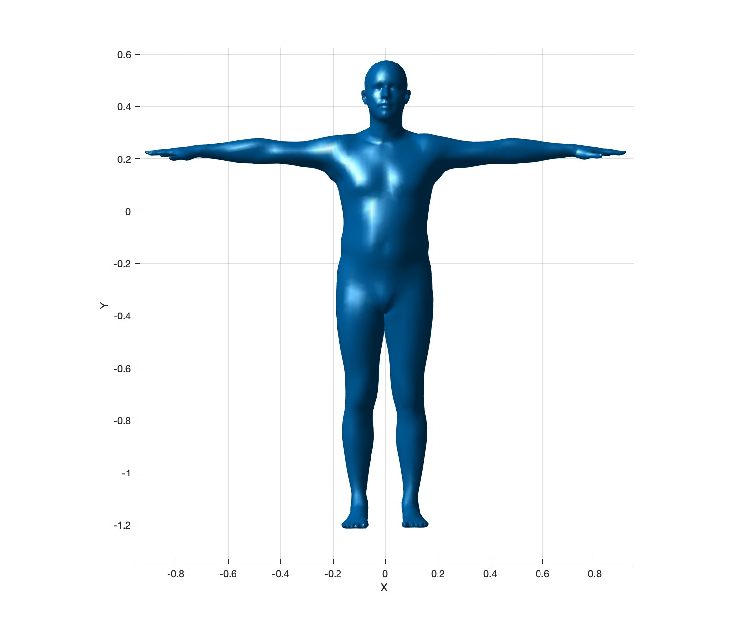
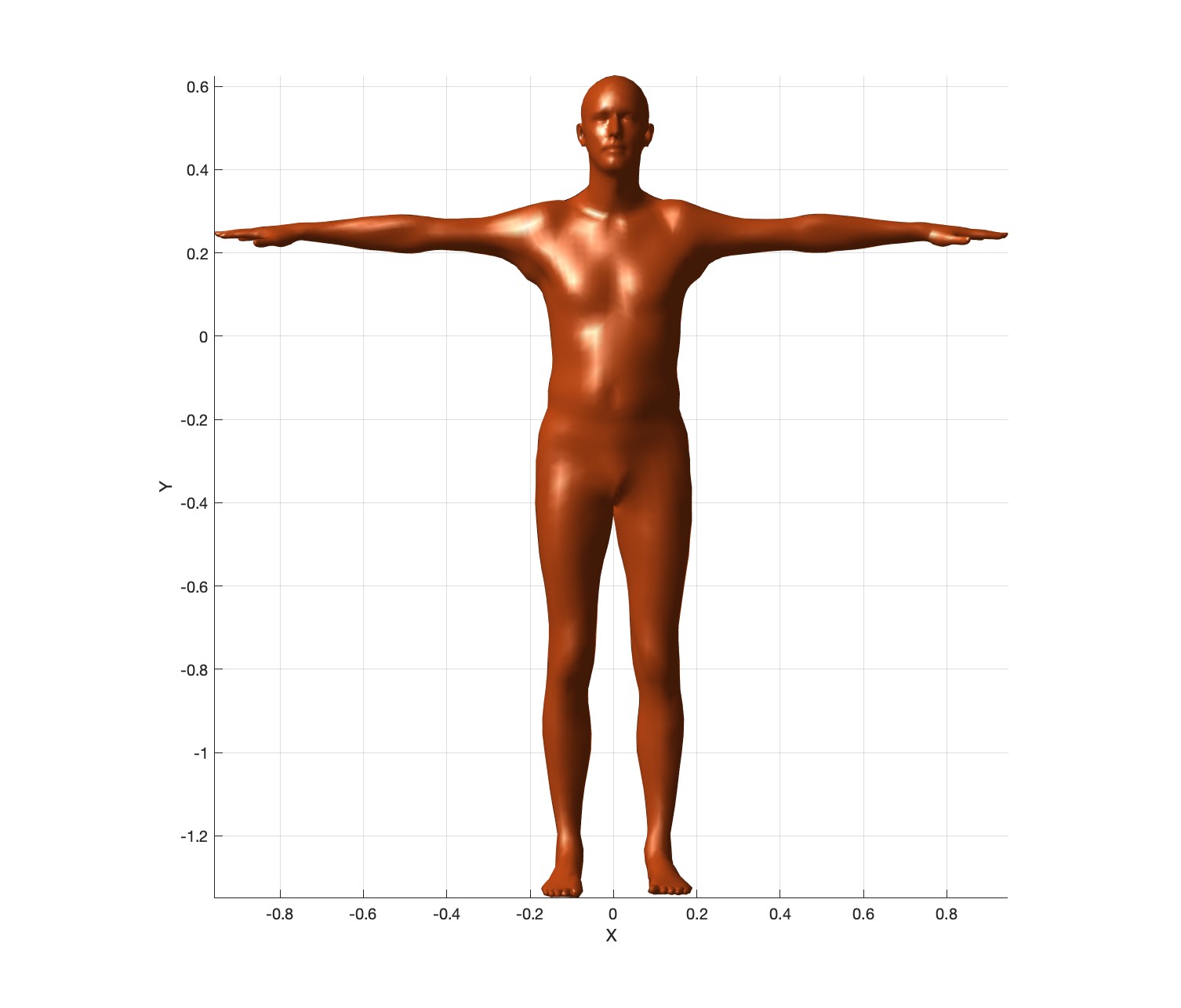
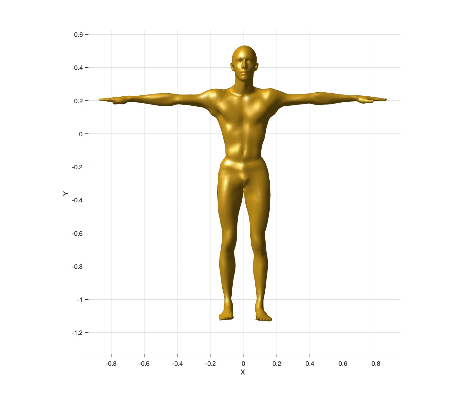
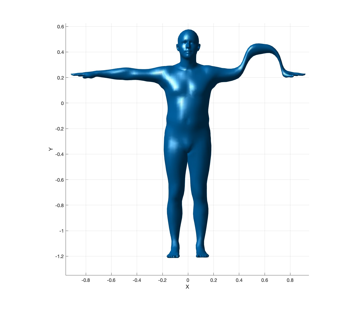
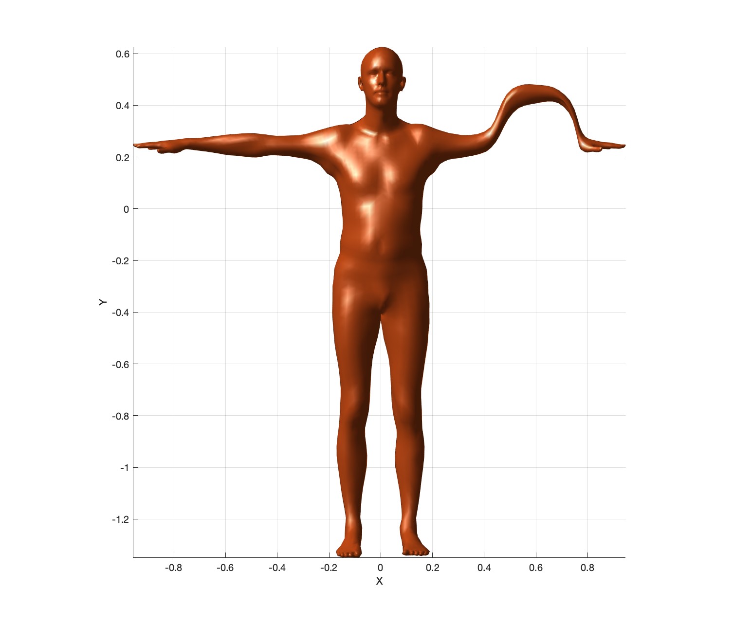
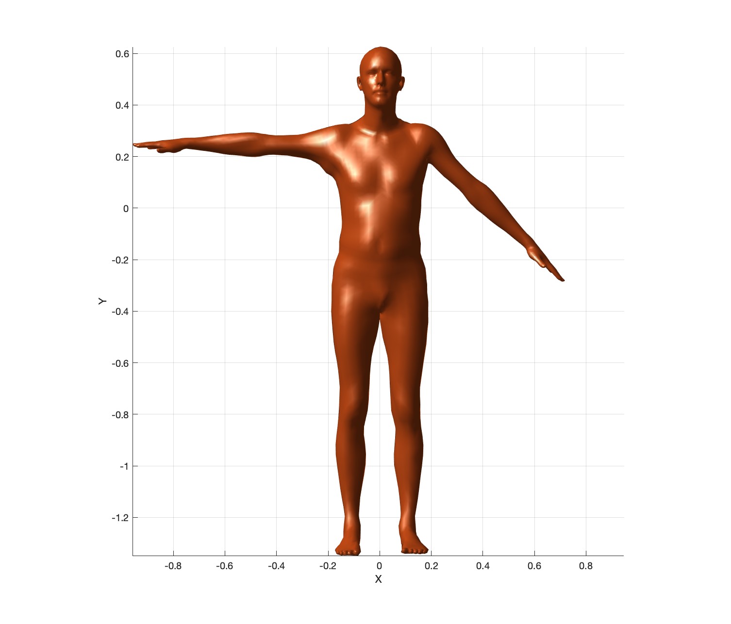
Then use the following two sets of \(\beta\)s to generate two meshes.
beta1 = [-1.711935 2.352964 2.285835 -0.073122 1.501402 -1.790568 -0.391194 2.078678 1.461037 2.297462];
beta2 = [1.573618 2.028960 -1.865066 2.066879 0.661796 -2.012298 -1.107509 0.234408 2.287534 2.324443];
Below, the original mesh (with \(\beta=0\)) is shown in blue. The red and yellow meshes correspond to the two \(\beta\) values above. (The colors are added just for visualization purposes; you do not need to export the colors.) From here on, we’ll call these \(\beta^{(0)}\), \(\beta^{(1)}\), and \(\beta^{(2)}\). If we use \(\beta^{(1)}\), then the mesh can be computed as \(x_\beta = x_0 + \sum_b \beta^{(1)}_b \Delta x_b\) for \(b \in [1,10]\), and the result would be the red mesh below. Similarly, using \(\beta^{(2)}\) should generate the yellow mesh.
Export these three meshes to frame000.obj,
frame001.obj, and frame002.obj in the
output1 folder. You can test them against the solution by
running
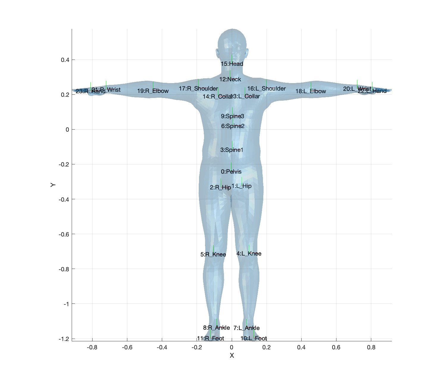
> ./objscmp2 ../output1 ../solution1Load smpl_skel00.txt. In this dataset, each of these
files contains the data corresponding to the bind pose of the base and
blendshape meshes. Each set of \(7\)
numbers corresponds to a bone; \(4\)
for the quaternion, and \(3\) for the
position. In this file, the quaternion can be ignored, since the
rotations are assumed to be identity for the bind pose. The indexing of
the bones for the bind pose is shown in the image below. (Note that
\(0\)-indexing is used for this
image.)
We now apply the absolute translations to the skeletons corresponding
to \(\beta^{(0)}\), \(\beta^{(1)}\), and \(\beta^{(2)}\). First load
smpl_skel01.txt through smpl_skel10.txt, which
contain the bone positions of the 10 blendshape meshes. These need to be
deformed to match the blue, red, and yellow meshes. This should be done
in the same way as before—create the delta bone positions by subtracting
the blendshapes: \(\Delta p_b = p_b -
p_0\) for \(b \in [1,10]\),
where \(p\) is the bone position. Then
add the weighted sum of these deltas to the base bone positions. For a
given \(\beta\), the bone positions
corresponding to the blendshape can be computed as \(p_\beta = p_0 + \sum_b \beta_b \Delta
p_b\).
After we have the skeleton for \(\beta^{(0)}\), \(\beta^{(1)}\), and \(\beta^{(2)}\), we are ready to apply
skinning. Load smpl_skin.txt, which contains the skinning
weights and influences. In this dataset, the maximum number of
influences is \(4\). Each line
corresponds to a vertex. For example, the first data line is
0 0.001881 4 0.000927 14 0.000877 15 0.996315and this tells us that vertex with index \(0\) is influenced by bones with indices \((0, 4, 14, 15)\) using weights \((0.001881, 0.000927, 0.000877, 0.996315)\), respectively. If skinning is implemented correctly, the resulting skinned meshes look the same as before, since we have not moved the skeleton yet.
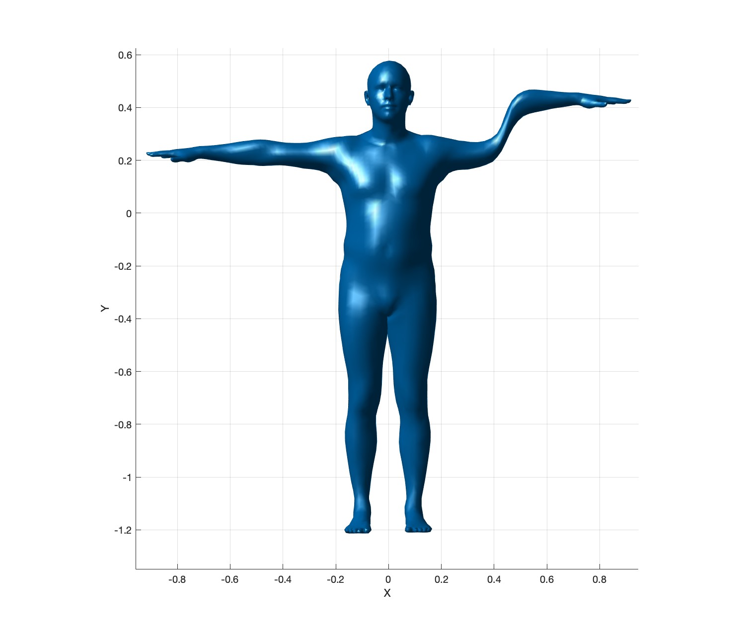
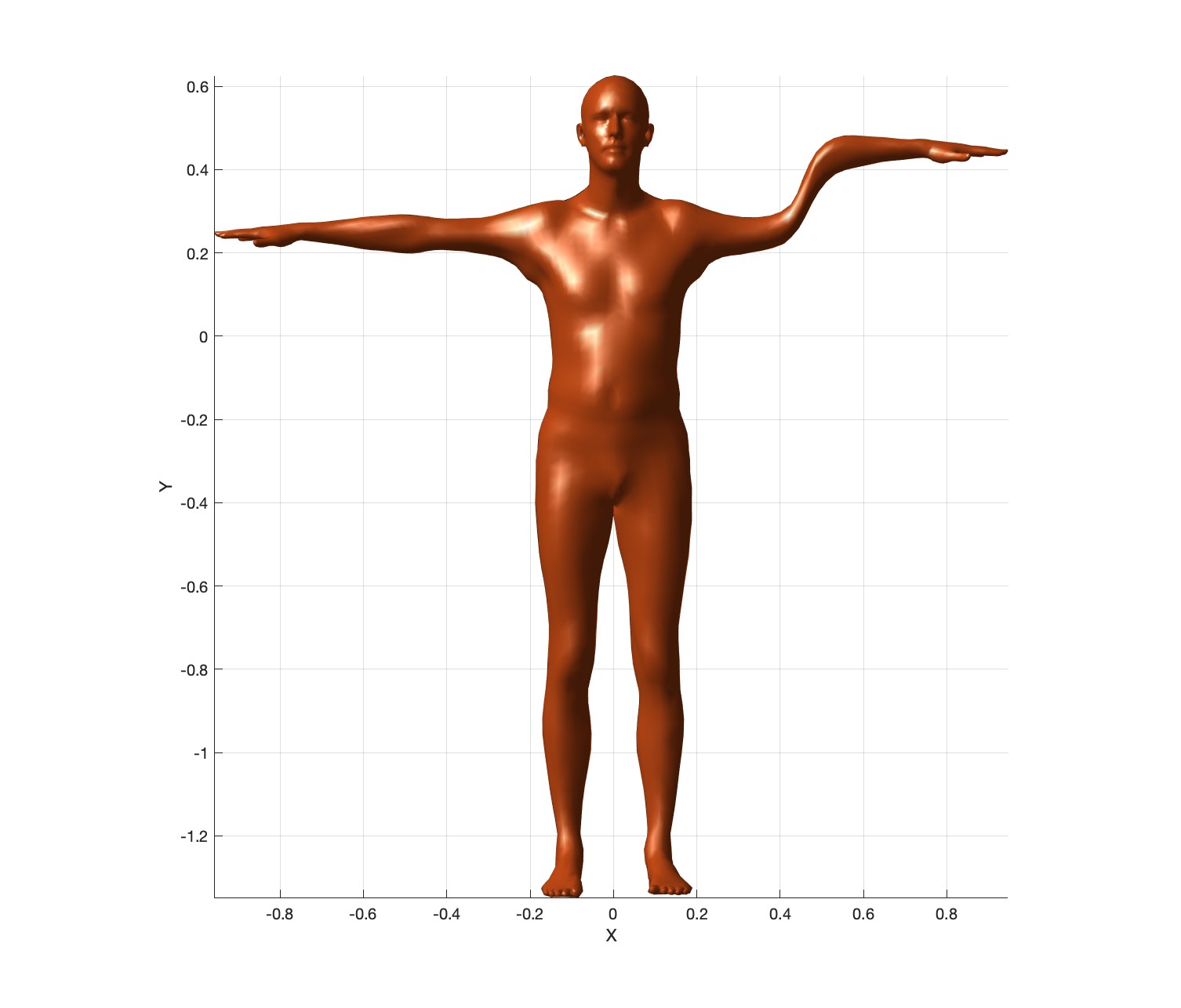
Now translate the “L_Elbow” bone by \(0.2\) units up in the Y-direction. Since the translation is not relative (not until the next task), the descendants of L_Elbow should not translate. Using \(\beta^{(0)}\), \(\beta^{(1)}\), and \(\beta^{(2)}\), the generated output should look like this:

Export these meshes as frame000.obj,
frame001.obj, and frame002.obj in the
output2 folder.
We now switch to relative translations. Load the hierarchy
information from smpl_hiearchy.txt and store the relative
translation of each bone with respect to its parent. For the root
(0:Pelvis), the relative and absolute translations should
be the same. Since the character’s skeletal hierarchy contains branching
structures, this product can be implemented efficiently with a
matrix stack. Once all the relative translations are computed,
the absolute translation of a bone can be reconstructed by
traversing the relative translations from the bone all the way to
the root (0:Pelvis). For example, the ancestors of
18:L_Elbow are: 16:L_Shoulder,
13:L_Collar, 9:Spine3, 6:Spine2,
3:Spine1, and 0:Pelvis. Therefore, the
absolute transformation for the left elbow can be reconstructed by
combining the relative transformations: \[
T = T_0 \, T_3 \, T_6 \, T_9 \, T_{13} \, T_{16} \, T_{18},
\] where the \(T_j\) are the
relative translation matrices. For example, for \(\beta^{(0)}\), the relative transforms for
the 0:Pelvis and 3:Spine1 are: \[
T_0 =
\begin{pmatrix}
1 & 0 & 0 & -0.0022 - 0\\
0 & 1 & 0 & -0.2408 - 0\\
0 & 0 & 1 & 0.0286 - 0\\
0 & 0 & 0 & 1
\end{pmatrix}
=
\begin{pmatrix}
1 & 0 & 0 & -0.0022\\
0 & 1 & 0 & -0.2408\\
0 & 0 & 1 & 0.0286\\
0 & 0 & 0 & 1
\end{pmatrix},
\] \[
T_3 =
\begin{pmatrix}
1 & 0 & 0 & 0.0023 - (-0.0022)\\
0 & 1 & 0 & -0.1164 - (-0.2408)\\
0 & 0 & 1 & -0.0098 - 0.0286\\
0 & 0 & 0 & 1
\end{pmatrix}
=
\begin{pmatrix}
1 & 0 & 0 & 0.0044\\
0 & 1 & 0 & 0.1244\\
0 & 0 & 1 & -0.0384\\
0 & 0 & 0 & 1
\end{pmatrix}.
\]
As in Task 2, translate the “L_Elbow” bone by \(0.2\) units up in the Y-direction. Once relative translations are used, the output should be as follows:
Export these meshes as frame000.obj,
frame001.obj, and frame002.obj in the
output3 folder.
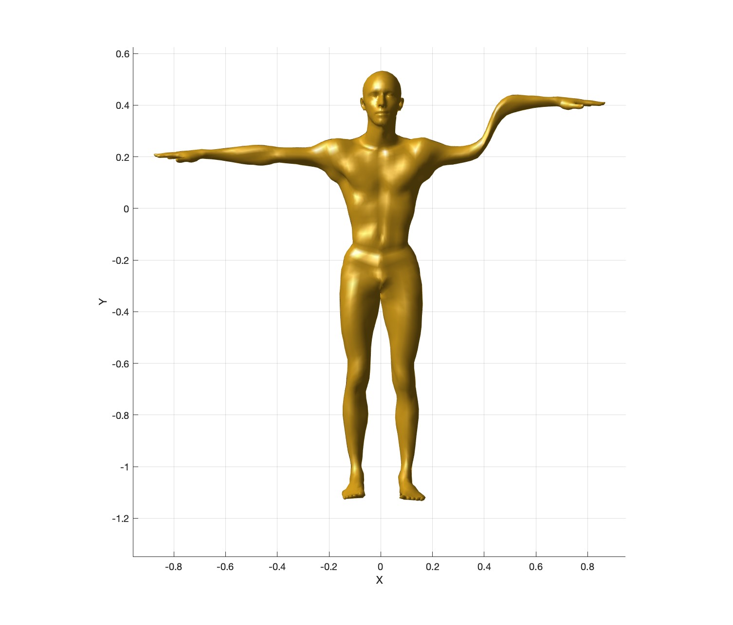
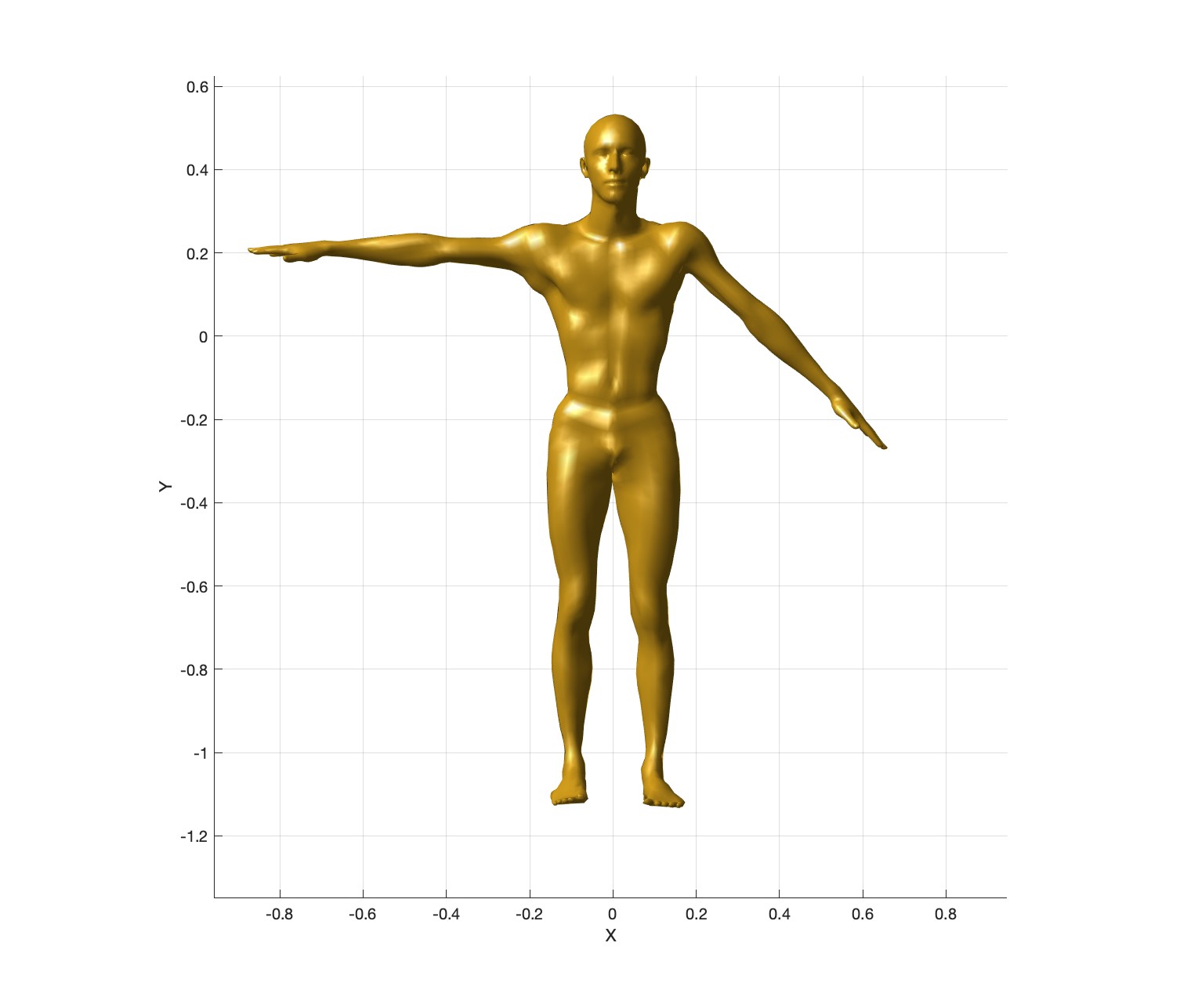
Now we switch to rotations. Each bone applies a relative translation with respect to its parent, and then a relative rotation. For example, the transformation for the left shoulder becomes: \[ T = T_0 \, R_0 \, T_3 \, R_3 \, T_6 \, R_6 \, T_9 \, R_9 \, T_{13} \, R_{13} \, T_{16} \, R_{16}, \] where the \(R_j\) are the relative rotation matrices. If the relative rotation matrices are all identity, the product is exactly the same as in Task 3.
Since the mocap data in the next task will use quaternions, we’ll use
quaternions for this task as well. Bend the shoulder by applying the
quaternion 0, 0, -0.3827, 0.9239. (Here, the quaternion is
ordered as \((x,y,z,w)\).) This
corresponds to a rotation about the Z-axis by \(-45\) degrees. Apply this rotation with
\(\beta\) set to \(\beta^{(0)}\), \(\beta^{(1)}\), and \(\beta^{(2)}\).
Here are some test numbers for \(\beta^{(0)}\) (the blue character):
The matrix for L_Collar is \(T = T_0 \, R_0 \, T_3 \, R_3 \, T_6 \, R_6 \, T_9
\, R_9 \, T_{13} \, R_{13}\). None of these joints have any
rotation, so all of the rotation matrices are identity. The translation
matrices are the local transltions from the previous task. The product
should be:
  1.0000         0         0    0.0762
       0    1.0000         0    0.1916
       0         0    1.0000    0.0010
       0         0         0    1.0000
The matrix for L_Shoulder is \(T = T_0 \, R_0 \, T_3 \, R_3 \, T_6 \, R_6 \, T_9
\, R_9 \, T_{13} \, R_{13} \, T_{16} \, R_{16}\). The only
rotation matrix that is not the identity is \(R_{16}\). The product should be:
  0.7071    0.7071         0    0.1991
 -0.7071    0.7071         0    0.2368
       0         0    1.0000   -0.0181
       0         0         0    1.0000
The matrix for L_Wrist is \(T = T_0 \, R_0 \, T_3 \, R_3 \, T_6 \, R_6 \, T_9
\, R_9 \, T_{13} \, R_{13} \, T_{16} \, R_{16} \, T_{20} \,
R_{20}\). The only rotation matrix that is not the identity is
\(R_{16}\). The product should be:
  0.7071    0.7071         0    0.5655
 -0.7071    0.7071         0   -0.1337
       0         0    1.0000   -0.0484
       0         0         0    1.0000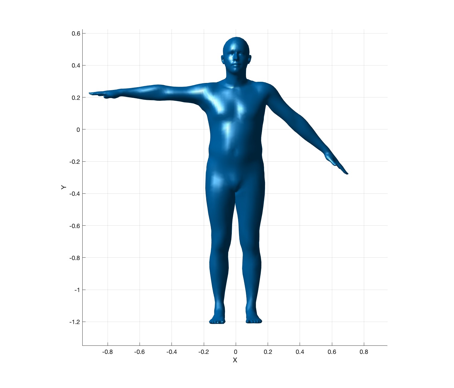
Export these meshes as frame000.obj,
frame001.obj, and frame002.obj in the
output4 folder.
Load smpl_quaternions_mosh_cmu_7516.txt. This file has
160 frames, and each data line corresponds to a frame. The first 3
numbers are the root translations, which can be ignored for this
assignment. The remaining numbers are the quaternions \((x,y,z,w)\) for the 24 bones. Each
quaternion represents the relative rotation of a joint with respect to
its parent joint.
Using the three sets of \(\beta\)
values (\(\beta^{(0)}\), \(\beta^{(1)}\), and \(\beta^{(2)}\)), play back the animation
sequentially. Since there are 160 frames, the total number of obj files
generated should be 480. These files should be exported as
frame000.obj through frame479.obj in the
output5 folder. (Note that in the figure title, the
animation index and frame index use \(1\)-indexing, whereas the obj filename uses
\(0\)-indexing.)

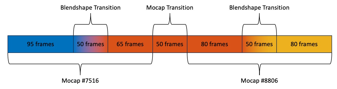
For the final task, generate the following output. (Note that in the figure title, the animation index and frame index use \(1\)-indexing, whereas the obj filename uses \(0\)-indexing.) As a reminder, to linearly interpolate between two quantities \(x_0\) and \(x_1\), use \((1-\alpha) x_0 + \alpha x_1\), where \(\alpha \in [0,1]\). In this task, linear interpolation is performed over 50 frames. On the first frame, \(\alpha\) should be \(0\), and on the 50th frame, \(\alpha\) should be \(1\).
We are now using both animations
(smpl_quaternions_mosh_cmu_7516.txt and
smpl_quaternions_mosh_cmu_8806.txt).
frame000.obj through
frame094.obj in the output6 folder.frame095.obj through
frame144.obj.frame145.obj through
frame209.obj.frame210.obj through
frame259.obj.frame260.obj through
frame339.obj.frame340.obj through
frame389.obj.frame390.obj through
frame469.obj.The summary is shown below.
Here is a nicely rendered version by Utsawb Lamichhane [2025].
output1)output2)output3)output4)output5)output6)Total: 100 points.
Failing to follow these points may decrease your “general execution” score.
cmake,
make, … must work to compile the source.
A3 <TASK#>, where the
argument is the task number 1 … 6.python A3.py <TASK#>, where
the argument is the task number 1 … 6.A3(<TASK#>), where the
argument is the task number 1 … 6.output1 …
output6 exist. Your code must be able to create these
folders if needed.(*.~)(*.o)(.vs)(.git)UIN.zip (e.g.,
12345678.zip).UIN/ (e.g. 12345678/).src/,
CMakeLists.txt, etc..zip format (not .gz,
.7z, .rar, etc.).