In this lab, we’re going to construct a couple of cubics that satisfy a set of user supplied constraints.
Please download the lab and go over the code.
For solving a linear system, we are using a C++ library called Eigen. You’ll have to install this in the same way you installed glm in lab 0. You’ll need to create a new environment variable called EIGEN3_INCLUDE_DIR that points to the Eigen directory. Once you have it installed, you may want to look at this quick tutorial.
Your first task is to draw the two cubics. The coefficients of the two cubics have already been set for you. These two sets of coefficients are stored in coeffs0 and coeffs1. (In the next task, you will be changing these coefficients.) Given these coefficients, the two cubics are given by:
\[ \begin{aligned} & f_0(x) = a_0 x^3 + b_0 x^2 + c_0 x + d_0,\\ & f_1(x) = a_1 x^3 + b_1 x^2 + c_1 x + d_1. \end{aligned} \]
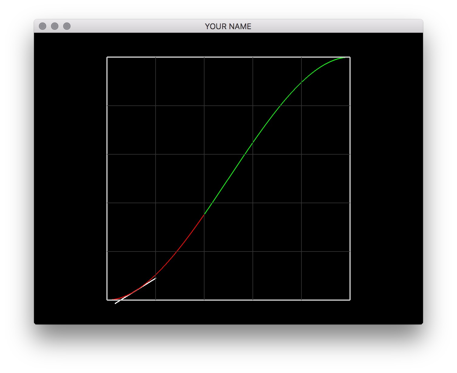
The coefficient vectors coeffs0 and coeffs1 store the \(4\) coefficients of the two cubics: \((a_0, b_0, c_0, d_0)\) and \((a_1, b_1, c_1, d_1)\) respectively. Use two different colors for the two cubics. The xmid global variable, which is set to \(0.4\), determines where the first cubic ends and the second cubic begins. (The first cubic goes from \(0.0\) to \(0.4\), and the second cubic goes from \(0.4\) to \(1.0\).)

Compute the coefficient vectors coeffs0 and coeffs1 that satisfy the following \(8\) constraints. Note that some of these conditions are on the function itself (\(f(x)\)), and some are on the derivative (\(f'(x)\)).
\[ \begin{aligned} & f_0(0.0) = 0.0,\\ & f'_0(0.0) = 0.0,\\ & f_0(0.4) = f_1(0.4),\\ & f'_0(0.4) = f'_1(0.4),\\ & f_1(0.5) = 0.2,\\ & f'_1(0.5) = 0.0,\\ & f_1(1.0) = 1.0,\\ & f'_1(1.0) = 0.0. \end{aligned} \]
You need to come up with the correct entries for \(A\) and \(b\) and then solve the linear system \(A c = b\) for \(c\). Here, \(A\) is \(8 \times 8\), and \(b\) and \(c\) are \(8 \times 1\). The top four elements of \(c\) are coeffs0, and the bottom four are coeffs1. With Eigen, you can use the following to solve a linear system.
VectorXf c = A.colPivHouseholderQr().solve(b);Once you get the correct coefficients, you’ll see the figure below.

Finally, draw the tangent line of the functions using the x-coord of the mouse. The global variable, mouse, contains the world coordinates of the mouse cursor. Evaluate the position and the derivative of the function at \(x\) (stored in mouse(0)) and draw a line that touches the function tangentially. When the mouse moves, this line should move with it. You’ll need to use the derivative, \(f'(x)\), for this. Remember that \(f'(x)\) gives the “rise over run” of the function. You should normalize the displayed tangent vector.