Due Thursday, 10/26 at 23:59:59. You must work individually.
In this assignment, you will be implementing inverse kinematics with your own nonlinear optimizers:
The first part of the assignment (Tasks A.\(1\)-A.\(5\)) will be on writing the optimizers and testing them with the Rosenbrock function. The second part of the assignment (Tasks B.\(1\)-B.\(5\)) will be on using these optimizers on inverse kinematics.
For IK (Task B), grades will be given out depending on how far you get along in the assignment. For example, if your program works with \(4\) links, then you will get full points for the \(1\)- and \(2\)-link tasks. Here is an example with \(10\) links:
You may work in C++ or Python.
EIGEN3_INCLUDE_DIR that points to the Eigen directory. Once you have it installed, you may want to look at this quick tutorial.To run tasks A.1-A.5 (Rosenbrock):
> ./A4 <RESOURCE_DIR> A.xThe last argument can be A.1 through A.5.
To run tasks B.1-B.5 (IK):
> ./A4 <RESOURCE_DIR> B.xThe last argument can be B.1 through B.5.
Optionally, you can run the built-in OpenGL visualizer for IK by supplying an additional argument at the end:
> ./A4 <RESOURCE_DIR> B.x 1double instead of float.To run tasks A.1-A.5 (Rosenbrock)
> python A4.py <RESOURCE_DIR> A.xThe last argument can be A.1 through A.5.
To run tasks B.1-B.5 (IK)
> python A4.py <RESOURCE_DIR> B.xThe last argument can be B.1 through B.5.
float type, which has 64 bits of precision.We will be using the Rosenbrock function as the objective: \[ \displaylines{ f(\vec{x}) = (a-x_0)^2 + b(x_1-x_0^2)^2\\ \vec{g}(\vec{x}) = 2 \begin{pmatrix} -(a-x_0) - 2bx_0(x_1-x_0^2)\\ b(x_1-x_0^2) \end{pmatrix}\\ H(\vec{x}) = 2 \begin{pmatrix} 2b(3x_0^2 - x_1) + 1 & -2bx_0\\ -2bx_0 & b \end{pmatrix} } \] with \(a=1\) and \(b=1\). The minimum is at \(\vec{x} = (1 \;\; 1)^\top\).

There are three eval() methods in the class ObjectiveRosenbrock. The first one returns just the objective value, the second one returns the objective and the gradient, and the third one returns the objective, gradient, and Hessian. Fill these methods to compute the expression given above. With the input argument \(\vec{x} = (-1 \;\; 0)^\top\), the returned values should be: \[
\displaylines{
f(\vec{x}) = 5\\
\vec{g}(\vec{x}) =
\begin{pmatrix}
-8\\
-2
\end{pmatrix}\\
H(\vec{x}) =
\begin{pmatrix}
14 & 4\\
4 & 2
\end{pmatrix}.
}
\] Running A4 <RESOURCE_DIR> A.1 should write these values to resources/outputA1.txt:
5
-8
-2
14  4
 4  2
The first line is for \(f(\vec{x})\), the next two lines are for \(\vec{g}(\vec{x})\), and the last two lines are for \(H(\vec{x})\). With Eigen, the vector and matrix classes have operator<< defined, so you can simply write output << x << endl; to write the variable x to the stream output.
Implement the following pseudocode in OptimizerGD.cpp:
for iter = 1 : iterMax
    % Search direction
    Evaluate f and g at x
    p = -g
    % Step
    Δx = α*p
    x += Δx
    if |g| < ε
        break
    end
end
Use \(\varepsilon=10^{-6}\), and \(\alpha=10^{-1}\). Start the search at \(\vec{x} = (-1 \;\; 0)^\top\). After one iteration, \(\vec{x}\) should be \((-0.2 \;\; 0.2)^\top\). Now set iterMax=50. Running the command A4 <RESOURCE_DIR> A.2 should write the number of iterations and the computed \(\vec{x}\) to resources/outputA2.txt:
50
0.943086
0.864814
(The number of iterations may be off by \(1\) depending on \(0\)-indexing or \(1\)-indexing is used.)
The choice of \(\alpha\) matters a lot. Setting it to be \(1.0\), for example, makes the optimizer diverge. We thus turn our attention next to line search.
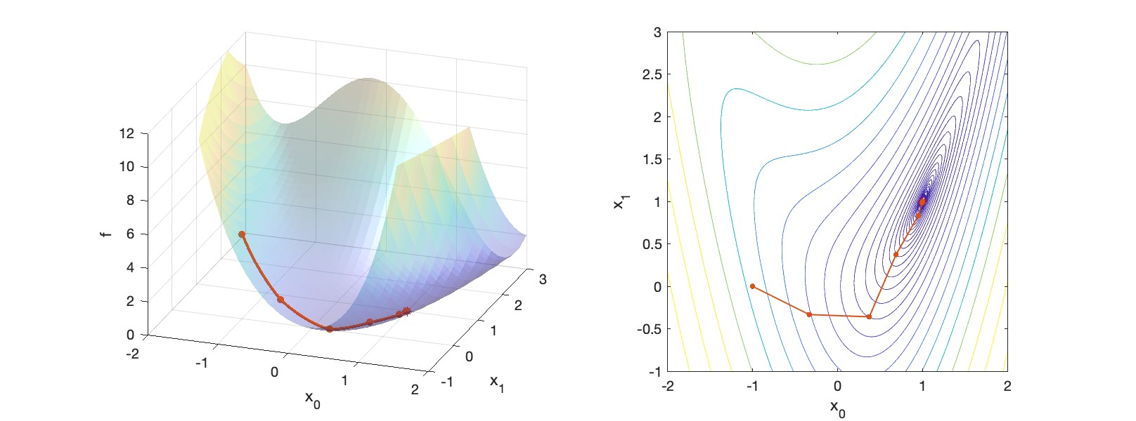
Modify OptimizerGD.cpp to implement the following pseudocode:
for iter = 1 : iterMax
    % Search direction
    Evaluate f and g at x
    p = -g
    % Line search
    α = α0
    for iterLS = 1 : iterMaxLS
        Δx = α*p
        Evaluate f1 at x + Δx
        if f1 < f
            break
        end
        α *= γ
    end
    % Step
    x += Δx
    if |g| < ε
        break
    end
end
Use iterMax=50, \(\varepsilon=10^{-6}\), \(\alpha_{0}=1\), \(\gamma=0.8\), and iterMaxLS=20. Start the search at \(\vec{x} = (-1 \;\; 0)^\top\). Running A4 <RESOURCE_DIR> A.3 should write the number of outer iterations and the computed \(\vec{x}\) to resources/outputA3.txt:
50
0.990237
0.981615
(The number of iterations may be off by \(1\) depending on \(0\)-indexing or \(1\)-indexing is used.)
Gradient descent is slow to converge, especially near the solution. We thus turn to Newton’s Method next.
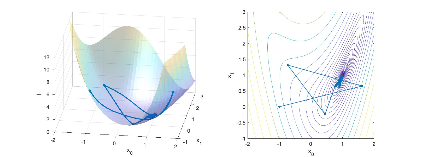
Implement the following pseudocode in OptimizerNM.cpp:
for iter = 1 : iterMax
    % Search direction
    Evaluate f, g, and H at x
    p = -H\g
    % Line search
    α = α0
    for iterLS = 1 : iterMaxLS
        Δx = α*p
        Evaluate f1 at x + Δx
        if f1 < f
            break
        end
        α *= γ
    end
    % Step
    x += Δx
    if |g| < ε
        break
    end
end
The notation x = A\b is the MATLAB notation for solving the linear system \(Ax=b\). It is important to use an appropriate numerical solver for this operation. (Do not use the inverse!) Assuming that Hessian is symmetric positive definite (nice and convex), we can use Eigen’s LDLT solver: x = A.ldlt().solve(b).
Use iterMax=50, \(\varepsilon=10^{-6}\), \(\alpha_{0}=1\), \(\gamma=0.8\), and iterMaxLS=20. Start the search at \(\vec{x} = (-1 \;\; 0)^\top\). Running A4 <RESOURCE_DIR> A.4 should write the number of outer iterations and the computed \(\vec{x}\) to resources/outputA4.txt:
8
1.000000
1.000000
(The number of iterations may be off by \(1\) depending on \(0\)-indexing or \(1\)-indexing is used.)
Newton’s Method is fast to converge, especially near the solution. However, forming the Hessian matrix and solving with it can become the bottleneck. We thus turn to BFGS next.
Implement the following pseudocode in OptimizerBFGS.cpp:
A = I
x0 = 0
g0 = 0
for iter = 1 : iterMax
    % Search direction
    Evaluate f and g at x
    if iter > 1
        s = x - x0
        y = g - g0
        ρ = 1/(y'*s)
        A = (I - ρ*s*y')*A*(I - ρ*y*s') + ρ*s*s'
    end
    p = -A*g
    % Line search
    α = α0
    for iterLS = 1 : iterMaxLS
        Δx = α*p
        Evaluate f1 at x + Δx
        if f1 < f
            break
        end
        α *= γ
    end
    % Step
    x0 = x
    g0 = g
    x += Δx
    if |g| < ε
        break
    end
end
Use iterMax=50, \(\varepsilon=10^{-6}\), \(\alpha_{0}=1\), \(\gamma=0.8\), and iterMaxLS=20. Start the search at \(\vec{x} = (-1 \;\; 0)^\top\). Running A4 <RESOURCE_DIR> A.5 should write the number of outer iterations and the computed \(\vec{x}\) to resources/outputA5.txt:
12
1.000000
1.000000
(The number of iterations may be off by \(1\) depending on \(0\)-indexing or \(1\)-indexing is used.)

From this point on, do not modify your optimizers. The goal of the next set of tasks is all about coming up with a new objective function for IK.
Take a look at the Link class. It has the following member variables:
int for the “depth” of the link, with the root having index \(0\).Vector2d representing the XY position \(\vec{t}\) of the link joint wrt the parent joint. For this assignment, we will assume that \(\vec{t} = (1 \;\; 0)^\top\) for all joints other than the root. The root is at the origin, so \(\vec{t} = (0 \;\; 0)^\top\).double for the current angle, \(\theta\). This is what IK will optimize. In other words, this is the \(\vec{x}\) that the optimizer takes in.Matrix4d, \(^i_{Mi}E\), for the transform of the mesh with respect to this link joint. This is only used for visualizing the mesh.The length of each link is implicitly set to \(1\). Since this is a 2D planar mechanism, only a single scalar is needed for the rotation. For convenience, the origin of each link is going to be where the joint is. For example, for the “upper arm” link, the origin will be at the shoulder, and for the “lower arm” link the origin is going to be at the elbow. Using the position \(\vec{p}\) and the rotation \(\theta\) member variables, the transformation matrix from the parent link’s joint to this link’s joint is: \[ ^p_iE(\theta) = T(\vec{t}) R(\theta). \] The leading superscript \(p\) is for “parent” (not “position”), and the leading subscript \(i\) is for the ith body.
We will start slowly. First, we will solve inverse kinematics with only \(1\) joint using GD or BFGS. We will define the objective function \(f(\theta)\) and its gradient \(g(\theta)\), and then use the optimizers you wrote in the previous task. The Hessian \(H(\theta)\) takes a bit of extra work, so we will leave it for later.

Each link is of length \(1.0\), so place an end-effector \(\vec{r}\) in the local coordinate space of the link at \((1,0)\). Keep in mind that there should be a homogeneous coordinate of \(1\) for this point. In your code, it is a good idea to use Vector3d instead of Vector2d and explicitly store the homogeneous coordinate. Once \(\vec{p}\), \(\vec{p}'\), and \(\vec{p}''\) are computed, it is ok to drop the homogeneous coordinate from these quantities.
The world-space position, \(\vec{p}\), of the end-effector and its derivatives are: \[ \displaylines{ \vec{p}(\theta) = T R(\theta) \vec{r}\;\\ \vec{p}'(\theta) = T R'(\theta) \vec{r}\;\\ \vec{p}''(\theta) = T R''(\theta) \vec{r}, } \] where \(T\) is the usual 2D translation matrix: \[ T = \begin{pmatrix} 1 & 0 & \vec{t}_x\\ 0 & 1 & \vec{t}_y\\ 0 & 0 & 1 \end{pmatrix}, \] and \(R(\theta)\) is the usual rotation matrix about the Z-axis: \[ \displaylines{ R(\theta) = \begin{pmatrix} \cos(\theta) & -\sin(\theta) & 0\\ \sin(\theta) & \cos(\theta) & 0\\ 0 & 0 & 1 \end{pmatrix}\;\;\,\\ R'(\theta) = \begin{pmatrix} -\sin(\theta) & -\cos(\theta) & 0\\ \cos(\theta) & -\sin(\theta) & 0\\ 0 & 0 & 0 \end{pmatrix}\,\\ R''(\theta) = \begin{pmatrix} -\cos(\theta) & \sin(\theta) & 0\\ -\sin(\theta) & -\cos(\theta) & 0\\ 0 & 0 & 0 \end{pmatrix}. } \] The second derivative, \(\vec{p}''(\theta)\) and \(R''(\theta)\), will not be needed until we use Newton’s Method in Task B.5.
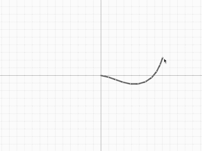
In the original rest state (figure above), the numerical values for the \(1\)-link system are (homogeneous coordinate not shown): \[ \displaylines{ \vec{p}(\theta) = \begin{pmatrix} 1 \\ 0 \end{pmatrix}\;\;\\ \vec{p}'(\theta) = \begin{pmatrix} 0 \\ 1 \end{pmatrix}\;\;\,\\ \vec{p}''(\theta) = \begin{pmatrix} -1 \\ 0 \end{pmatrix}. } \]
For Gradient Descent and BFGS, we need the objective function value \(f(\theta)\) and its gradient, \(\vec{g}(\theta)\). (Remember, we don’t need the Hessian, \(H(\theta),\) until we get to Newton’s Method.) The objective value is \[ \displaylines{ f(\theta) = \frac{1}{2} w_\text{tar} \Delta \vec{p}^\top \Delta \vec{p} + \frac{1}{2} w_\text{reg} \theta^2\\ \Delta \vec{p} = \vec{p}(\theta) - \vec{p}_\text{target}.\qquad\qquad\;\; } \]
The two weights, \(w_\text{tar}\) and \(w_\text{reg}\), can be set to arbitrary positive values, depending on the desired strength of the “targeting” energy and the “regularizer” energy.
For now, you can use \(w_\text{tar} = 1e3\) and \(w_\text{reg} = 1e0\).
The gradient is a scalar for this \(1\)-link task: \[ g(\theta) = w_\text{tar} \Delta \vec{p}^\top \vec{p}' + w_\text{reg} \theta. \] The Hessian (not needed yet) is also a scalar for this \(1\)-link task: \[ H(\theta) = w_\text{tar} (\vec{p}'^\top \vec{p}' + \Delta \vec{p}^\top \vec{p}'') + w_\text{reg}. \] With the initial angle set to \(\theta = 0\), and with the goal position set to \(\vec{p}_\text{target} = (0 \;\; 1)^\top\), you should get the following values: \[ f(\theta) = 1000, \quad g(\theta) = -1000, \quad H(\theta) = 1. \]
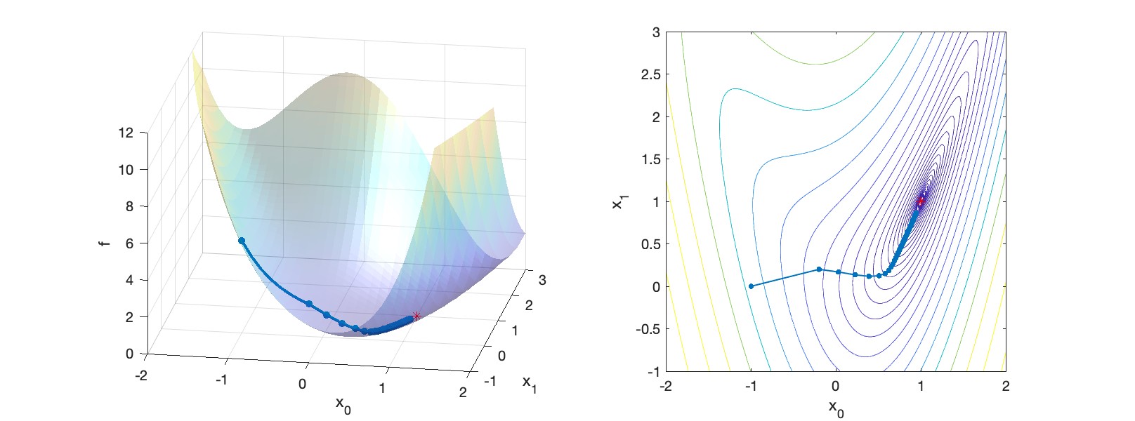
Run BFGS with the following settings:
1e31e051e-6201.00.5The returned answer should be close to \(\theta = \pi/2\). (See Wrapping \(\theta\) below.) Write the final angle to resources/outputB1.txt:
1.56295Note that Gradient Descent takes longer to converge. For example, it gives 1.49157 after 5 iterations.
If you’re using C++, the skeleton code comes with a built-in visualizer. The code is set up so that pressing the space bar toggles between forward kinematics and inverse kinematics.
. and , keys.r key should reset all the angles to 0.0.Since the minimization variables are joint angles, these variables may wrap around beyond (clockwise or counterclockwise) many times over. To prevent this, wrap the angles to be between \(-\pi\) and \(+\pi\) after each call to the optimizer with the following pseudocode. (Remember that you should not modify your optimizers after finishing Task A.)
while angle > pi
    angle -= 2*pi
while angle < -pi
angle += 2*piOne of the biggest sources of bugs is the derivatives, so it is helpful to have a routine that tests them against finite differences. To test the gradient vector, use the following pseudocode inside the main loop of GD. (This testing code should be commented out once testing is finished.)
e = 1e-7;
g_ = zeros(n,1);
for i = 1 : n
    theta_ = theta;
    theta_(i) += e;
    f_ = objective(theta_);
    g_(i) = (f_ - f)/e;
This pseudocode works in any number of dimensions (including the scalar case \(n=1\)). The finite differenced version of the gradient, g_, should closely match the analytical version of the gradient, g (at least within 1e-3 or so).
Once the gradient has been tested, use the following pseudocode inside the main loop of NM to test the Hessian matrix. (This testing code should be commented out once testing is finished.)
e = 1e-7;
H_ = zeros(n, n);
for i = 1 : n
    theta_ = theta;
    theta_(i) += e;
    [f_,g_] = objective(theta_);
    H_(:,i) = (g_ - g)/e;
The H_(:,i) notation above means the ith column of the matrix. With Eigen, this can be written as H_.col(i) = .... The finite differenced version of the Hessian, H_, should closely match the analytical version of the Hessian, H.
Next, we’re going to write a version that supports \(2\) links. If you’re feeling ambitious, you can skip to the \(4\)-link or the \(n\)-link tasks.
With two links, the minimization variable, \(\vec{\theta}\), is now a vector. The world-space position, \(\vec{p}\), of the end-effector is: \[ \vec{p}(\vec\theta) = T_0 R_0(\theta_0) T_1 R_1(\theta_1) \vec{r}. \] The derivatives are no longer scalars. For the gradient, compute the derivatives of \(\vec{p}\), drop the homogeneous coordinate, and then form a matrix \(P'\) of size \(2 \times 2\) (or \(1 \times 2\) block vector of \(2 \times 1\) vectors): \[ \displaylines{ \vec{p}'_0 = T_0 R'_0(\theta_0) T_1 R_1(\theta_1) \vec{r}\\ \vec{p}'_1 = T_0 R_0(\theta_0) T_1 R'_1(\theta_1) \vec{r}\\ P'(\vec\theta) = \begin{pmatrix} \vec{p}'_0 & \vec{p}'_1 \end{pmatrix} \in \mathbb{R}^{2 \times 2}.\qquad\; } \] Similarly, for the Hessian, compute the second derivatives of \(\vec{p}\), drop the homogeneous coordinate, and then form a matrix \(P''\) of size \(4 \times 2\) (or \(2 \times 2\) block matrix of \(2 \times 1\) vectors): \[ \displaylines{ \vec{p}''_{00} = T_0 R''_0(\theta_0) T_1 R_1(\theta_1) \vec{r}\\ \vec{p}''_{01} = T_0 R'_0(\theta_0) T_1 R'_1(\theta_1) \vec{r}\\ \vec{p}''_{10} = T_0 R'_0(\theta_0) T_1 R'_1(\theta_1) \vec{r}\\ \vec{p}''_{11} = T_0 R_0(\theta_0) T_1 R''_1(\theta_1) \vec{r}\\ P''(\vec\theta) = \begin{pmatrix} \vec{p}''_{00} & \vec{p}''_{01} \\ \vec{p}''_{10} & \vec{p}''_{11} \end{pmatrix} \in \mathbb{R}^{4 \times 2}.\;\;\, } \]
The objective function, \(f(\vec\theta)\), is still a scalar. In fact, the objective function for an optimization problem always returns a scalar. Compared to the \(1\)-link case, the only difference is that \(\vec\theta\), the deviation of the current joint angles from the rest joint angles, is now a vector. Therefore, instead of squaring this difference, we take the dot product by itself (i.e., transpose and multiply). The second term is also an inner product but with a regularization matrix sandwiched in between: \[
f(\vec\theta) = \frac{1}{2} w_\text{tar} \Delta \vec{p}^\top \Delta \vec{p} + \frac{1}{2} \vec\theta^\top W_\text{reg} \vec\theta,
\] where \(W_\text{reg}\) is a diagonal matrix of regularization weights \[
W_\text{reg} =
\begin{pmatrix}
w_{\text{reg}_0} & 0 \\
0 & w_{\text{reg}_1}
\end{pmatrix}.
\] For now, set \(w_{\text{reg}_0}\) and \(w_{\text{reg}_1}\) to 1e0.
Now the gradient is a \(2 \times 1\) vector: \[ \displaylines{ \vec{g}(\vec\theta) = w_\text{tar} \left( \Delta \vec{p}^\top P' \right)^\top + W_\text{reg} \vec\theta \qquad\qquad\quad\;\\ = w_\text{tar} \begin{pmatrix} \Delta \vec{p}^\top \vec{p}'_0\\ \Delta \vec{p}^\top \vec{p}'_1 \end{pmatrix} + W_\text{reg} \begin{pmatrix} \theta_0\\ \theta_1 \end{pmatrix}. } \] And the Hessian is a \(2 \times 2\) matrix: \[ \displaylines{ H(\vec\theta) = w_\text{tar} \left( P'^\top P' + \Delta \vec{p}^\top \odot P'' \right)^\top + W_\text{reg}\qquad\qquad\qquad\qquad\qquad\qquad\quad\\ = w_\text{tar} \left( \begin{pmatrix} \vec{p}_0^{'\top} \vec{p}'_0 & \vec{p}_0^{'\top} \vec{p}'_1\\ \vec{p}_1^{'\top} \vec{p}'_0 & \vec{p}_1^{'\top} \vec{p}'_1 \end{pmatrix} + \begin{pmatrix} \Delta \vec{p}^\top \vec{p}''_{00} & \Delta \vec{p}^\top \vec{p}''_{01}\\ \Delta \vec{p}^\top \vec{p}''_{10} & \Delta \vec{p}^\top \vec{p}''_{11} \end{pmatrix} \right) + W_\text{reg}. } \]
The \(\odot\) symbol above is used to mean that \(\Delta \vec{p}\) is dotted with each vector element of \(P''\).
With the initial angle set to \(\vec{\theta} = (0 \;\; 0)^\top\), and with the goal position set to \(\vec{p}_\text{target} = (1 \;\; 1)^\top\), you should get the following values: \[ \vec{p}(\vec{\theta}) = \begin{pmatrix} 2\\ 0 \end{pmatrix}, \quad P'(\vec{\theta}) = \begin{pmatrix} 0 & 0\\ 2 & 1\\ \end{pmatrix}, \quad P''(\vec{\theta}) = \begin{pmatrix} -2 & -1\\ 0 & 0\\ -1 & -1\\ 0 & 0 \end{pmatrix}, \quad f(\vec{\theta}) = 1000, \quad \vec{g}(\vec{\theta}) = \begin{pmatrix} -2000\\ -1000 \end{pmatrix}, \quad H(\vec{\theta}) = \begin{pmatrix} 2001 & 1000\\ 1000 & 1 \end{pmatrix}. \]
Run BFGS with the same settings as before:
1e31e0 and 1e051e-6201.00.5Write the final angles to resources/outputB2.txt. The output should be:
-0.000994772
1.54115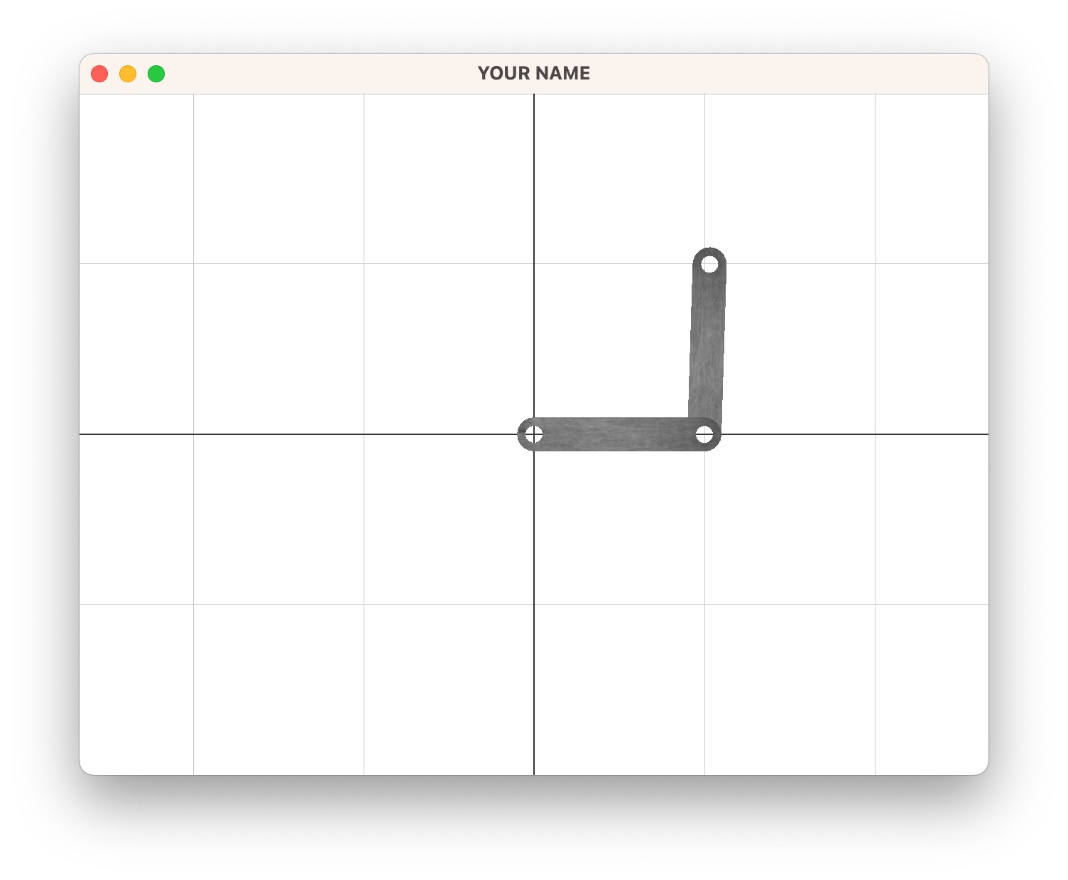
In this task, you’re going to hard code a \(4\)-link system, which follows the same steps as in the \(2\)-link system. If you’re feeling ambitious, you can skip this task and go straight to the \(n\)-link system.
If you skipped \(2\)-link IK, make sure to read the Wrapping and Debugging sections.
The minimization variable is now \(\vec\theta = (\theta_0 \;\; \theta_1 \;\; \theta_2 \;\; \theta_3)^\top\). The world-space position, \(\vec{p}\), of the end-effector is: \[ \vec{p}(\vec\theta) = T_0 R_0(\theta_0) T_1 R_1(\theta_1) T_2 R_2(\theta_2) T_3 R_3(\theta_3) \vec{r}. \] For the gradient, compute the derivatives of \(\vec{p}\), drop the homogeneous coordinate, and then form a matrix \(P'\) of size \(2 \times 4\) (or \(1 \times 4\) block vector of \(2 \times 1\) vectors): \[ \displaylines{ \vec{p}'_0 = T_0 R'_0(\theta_0) T_1 R_1(\theta_1) T_2 R_2(\theta_2) T_3 R_3(\theta_3) \vec{r}\\ \vec{p}'_1 = T_0 R_0(\theta_0) T_1 R'_1(\theta_1) T_2 R_2(\theta_2) T_3 R_3(\theta_3) \vec{r}\\ \vec{p}'_2 = T_0 R_0(\theta_0) T_1 R_1(\theta_1) T_2 R'_2(\theta_2) T_3 R_3(\theta_3) \vec{r}\\ \vec{p}'_3 = T_0 R_0(\theta_0) T_1 R_1(\theta_1) T_2 R_2(\theta_2) T_3 R'_3(\theta_3) \vec{r}\\ P'(\vec\theta) = \begin{pmatrix} \vec{p}'_0 & \vec{p}'_1 & \vec{p}'_2 & \vec{p}'_3 \end{pmatrix}.\qquad\qquad\qquad\qquad\quad\;\; } \] Similarly, for the Hessian, compute the second derivatives of \(\vec{p}\), drop the homogeneous coordinate, and then form a matrix \(P''\) of size \(8 \times 4\) (or \(4 \times 4\) block matrix of \(2 \times 1\) vectors): \[ \displaylines{ \vec{p}''_{00} = T_0 R''_0(\theta_0) T_1 R_1(\theta_1) T_2 R_2(\theta_2) T_3 R_3(\theta_3) \vec{r}\\ \vec{p}''_{01} = T_0 R'_0(\theta_0) T_1 R'_1(\theta_1) T_2 R_2(\theta_2) T_3 R_3(\theta_3) \vec{r}\\ \vec{p}''_{02} = T_0 R'_0(\theta_0) T_1 R_1(\theta_1) T_2 R'_2(\theta_2) T_3 R_3(\theta_3) \vec{r}\\ \vdots\\ \vec{p}''_{32} = T_0 R_0(\theta_0) T_1 R_1(\theta_1) T_2 R'_2(\theta_2) T_3 R'_3(\theta_3) \vec{r}\\ \vec{p}''_{33} = T_0 R_0(\theta_0) T_1 R_1(\theta_1) T_2 R_2(\theta_2) T_3 R''_3(\theta_3) \vec{r}\\ P''(\vec\theta) = \begin{pmatrix} \vec{p}''_{00} & \vec{p}''_{01} & \vec{p}''_{02} & \vec{p}''_{03}\\ \vec{p}''_{10} & \vec{p}''_{11} & \vec{p}''_{12} & \vec{p}''_{13}\\ \vec{p}''_{20} & \vec{p}''_{21} & \vec{p}''_{22} & \vec{p}''_{23}\\ \vec{p}''_{30} & \vec{p}''_{31} & \vec{p}''_{32} & \vec{p}''_{33} \end{pmatrix}.\qquad\qquad\qquad\quad\, } \]
The scalar objective function is: \[ f(\vec\theta) = \frac{1}{2} w_\text{tar} \Delta \vec{p}^\top \Delta \vec{p} + \frac{1}{2} \vec\theta^\top W_\text{reg} \vec\theta. \] The gradient, expressed as a column vector is: \[ \displaylines{ \vec{g}(\vec\theta) = w_\text{tar} \left( \Delta \vec{p}^\top P' \right)^\top + W_\text{reg} \vec\theta \qquad\qquad\qquad\quad\,\\ = w_\text{tar} \begin{pmatrix} \Delta \vec{p}^\top \vec{p}'_0\\ \Delta \vec{p}^\top \vec{p}'_1\\ \Delta \vec{p}^\top \vec{p}'_2\\ \Delta \vec{p}^\top \vec{p}'_3 \end{pmatrix} + W_\text{reg} \begin{pmatrix} \theta_0\\ \theta_1\\ \theta_2\\ \theta_3 \end{pmatrix}. } \] And the Hessian is a matrix: \[ \displaylines{ H(\vec\theta) = w_\text{tar} \left( P'^\top P' + \Delta \vec{p}^\top \odot P'' \right)^\top + W_\text{reg}\qquad\qquad\qquad\qquad\qquad\qquad\qquad\qquad\qquad\qquad\qquad\qquad\qquad\qquad\;\\ = w_\text{tar} \left( \begin{pmatrix} \vec{p}_0^{'\top} \vec{p}'_0 & \vec{p}_0^{'\top} \vec{p}'_1 & \vec{p}_0^{'\top} \vec{p}'_2 & \vec{p}_0^{'\top} \vec{p}'_3\\ \vec{p}_1^{'\top} \vec{p}'_0 & \vec{p}_1^{'\top} \vec{p}'_1 & \vec{p}_1^{'\top} \vec{p}'_2 & \vec{p}_1^{'\top} \vec{p}'_3\\ \vec{p}_2^{'\top} \vec{p}'_0 & \vec{p}_2^{'\top} \vec{p}'_1 & \vec{p}_2^{'\top} \vec{p}'_2 & \vec{p}_2^{'\top} \vec{p}'_3\\ \vec{p}_3^{'\top} \vec{p}'_0 & \vec{p}_3^{'\top} \vec{p}'_1 & \vec{p}_3^{'\top} \vec{p}'_2 & \vec{p}_3^{'\top} \vec{p}'_3 \end{pmatrix} + \begin{pmatrix} \Delta \vec{p}^\top \vec{p}''_{00} & \Delta \vec{p}^\top \vec{p}''_{01} & \Delta \vec{p}^\top \vec{p}''_{02} & \Delta \vec{p}^\top \vec{p}''_{03}\\ \Delta \vec{p}^\top \vec{p}''_{10} & \Delta \vec{p}^\top \vec{p}''_{11} & \Delta \vec{p}^\top \vec{p}''_{12} & \Delta \vec{p}^\top \vec{p}''_{13}\\ \Delta \vec{p}^\top \vec{p}''_{20} & \Delta \vec{p}^\top \vec{p}''_{21} & \Delta \vec{p}^\top \vec{p}''_{22} & \Delta \vec{p}^\top \vec{p}''_{23}\\ \Delta \vec{p}^\top \vec{p}''_{30} & \Delta \vec{p}^\top \vec{p}''_{31} & \Delta \vec{p}^\top \vec{p}''_{32} & \Delta \vec{p}^\top \vec{p}''_{33} \end{pmatrix} \right) + W_\text{reg}. } \]
The \(\odot\) symbol above is used to mean that \(\Delta \vec{p}\) is dotted with each vector element of \(P''\).
With the initial angle set to \(\vec{\theta} = (0 \;\; 0 \;\; 0 \;\; 0)^\top\), and with the goal position set to \(\vec{p}_\text{target} = (3 \;\; 1)^\top\), you should get the following values: \[ \displaylines{ \vec{p}(\vec{\theta}) = \begin{pmatrix} 4\\ 0 \end{pmatrix}, \quad P'(\vec{\theta}) = \begin{pmatrix} 0 & 0 & 0 & 0\\ 4 & 3 & 2 & 1 \end{pmatrix}, \quad P''(\vec{\theta}) = \begin{pmatrix} -4 & -3 & -2 & -1\\ 0 & 0 & 0 & 0\\ -3 & -3 & -2 & -1\\ 0 & 0 & 0 & 0\\ -2 & -2 & -2 & -1\\ 0 & 0 & 0 & 0\\ -1 & -1 & -1 & -1\\ 0 & 0 & 0 & 0 \end{pmatrix},\\ f(\vec{\theta}) = 1000, \quad \vec{g}(\vec{\theta}) = \begin{pmatrix} -4000\\ -3000\\ -2000\\ -1000 \end{pmatrix}, \quad H(\vec{\theta}) = \begin{pmatrix} 12000 & 9000 & 6000 & 3000\\ 9000 & 6001 & 4000 & 2000\\ 6000 & 4000 & 2001 & 1000\\ 3000 & 2000 & 1000 & 1 \end{pmatrix}. } \]
Run BFGS with the following settings. The only difference from before are the regularizer weights and the number of BFGS iterations.
1e301e0501e-6201.00.5Write the final angles to resources/outputB3.txt. The output should be:
-0.556147
0.519534
0.734012
0.477356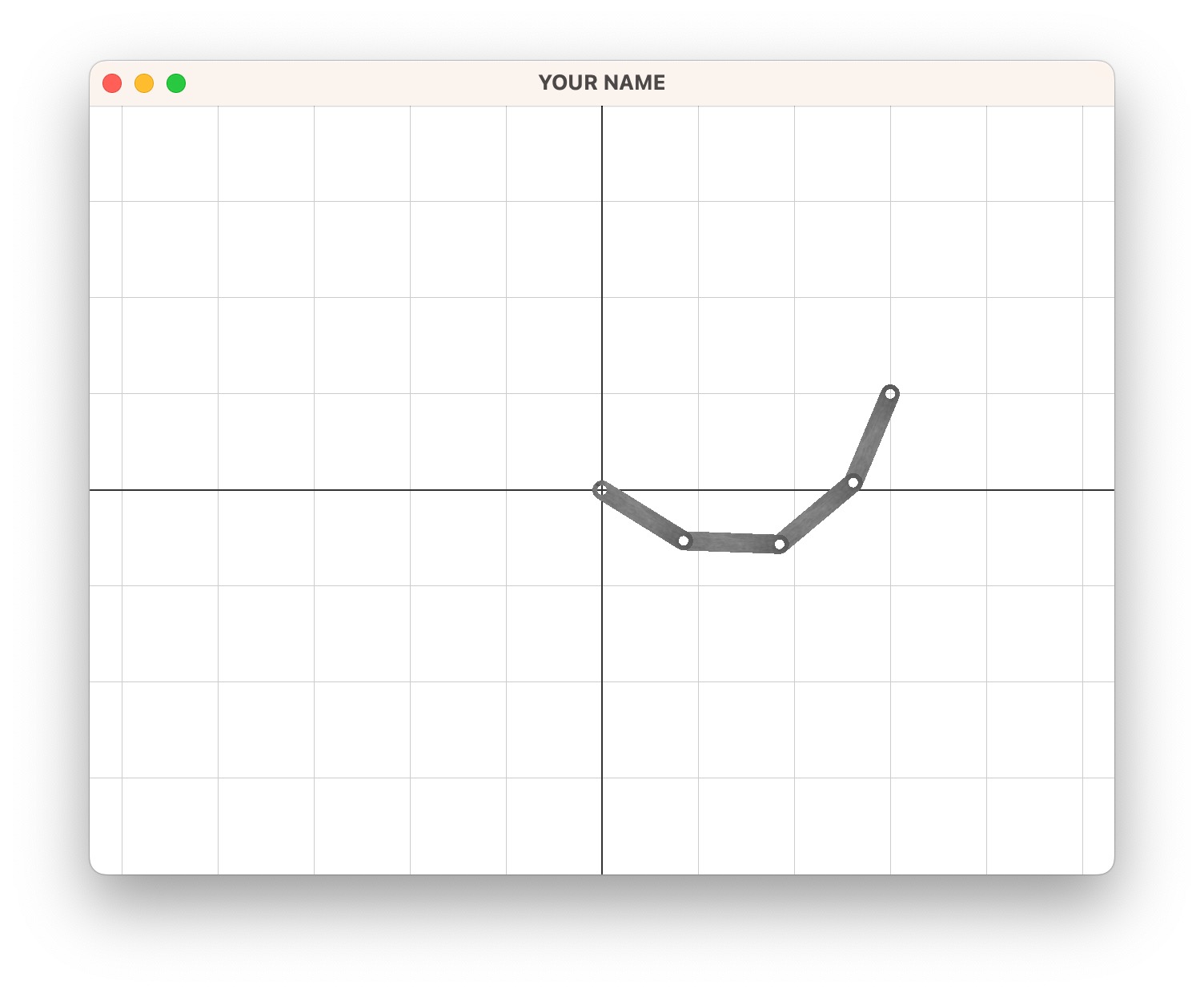
Convert your code to support an arbitrary number of links. Note that as you increase \(n\), the code will get slower and slower. Make sure to run your code in release mode. It is recommended that you first work on GD/BFGS and then NM.
If you skipped \(2\)-link IK, make sure to read the Wrapping and Debugging sections.
Run your code with the following settings. The only difference from before is the number of BFGS iterations:
10(9.0, 1.0)1e301e01501e-6201.00.5Your code should generate resources/outputB4.txt with the values for the 10 angles:
-0.502586
0.0591458
0.11322
0.157075
0.185851
0.195901
0.185851
0.157075
0.11322
0.0591458
Implement the Hessian calculation. Then run 2 iterations of BFGS followed by NM:
10(9.0, 1.0)1e301e021e-6201.00.5301e-6201.00.5Write the result to resources/outputB5.txt. This should produce the same result as the previous task but with fewer iterations. Observe that if we don’t start with BFGS, NM gets stuck in a local minimum.
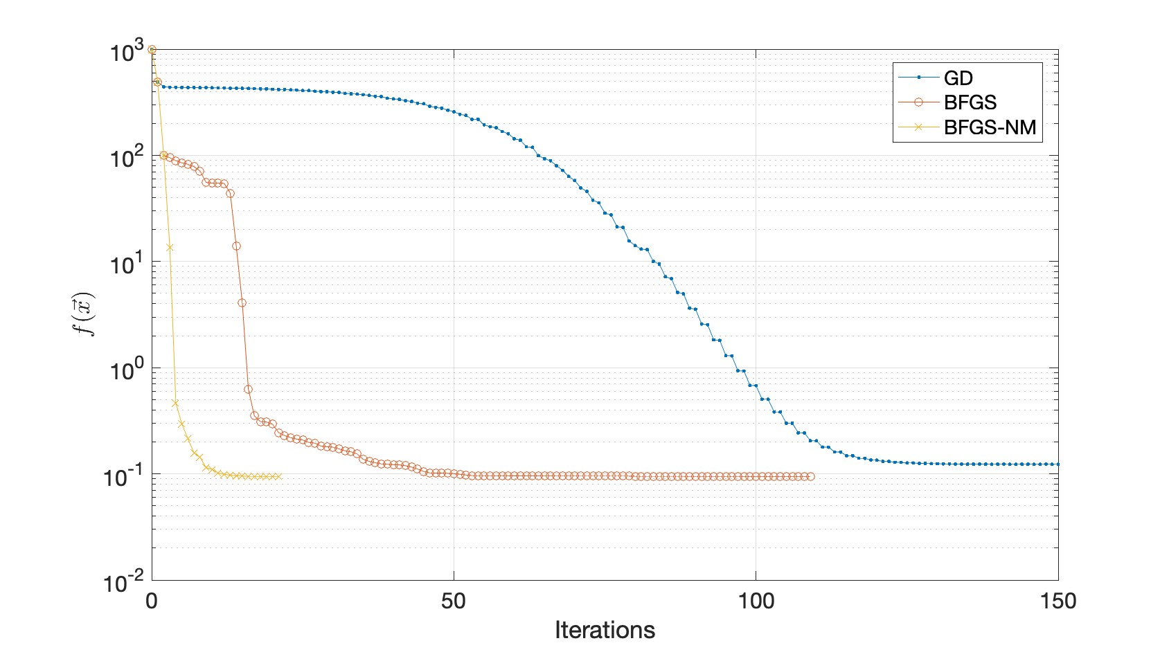
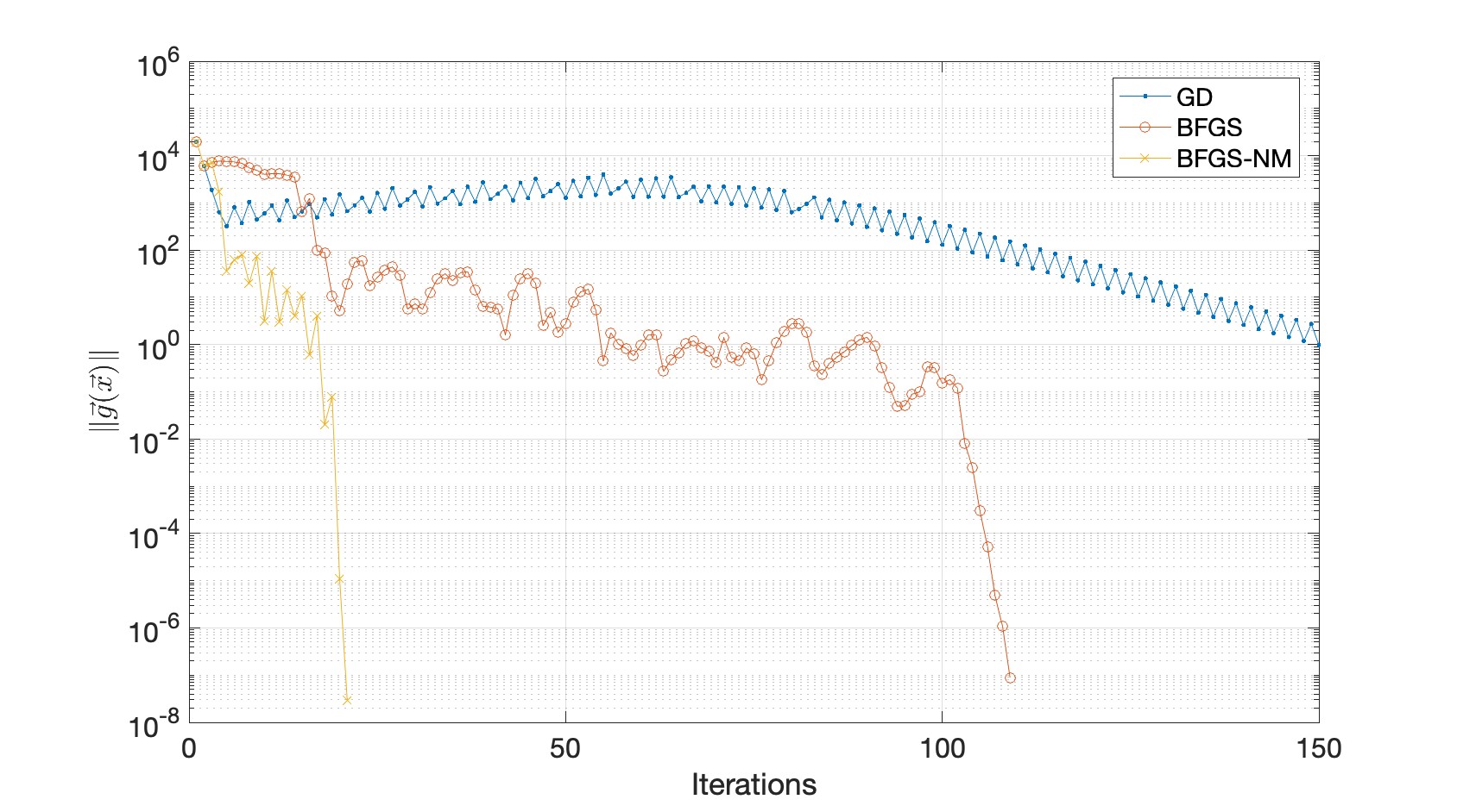
The following plots compare the three optimizers. The left plot shows how the objective decreases, and the right plot shows how the norm of the gradient decreases.
Total: 100 + 10 points
You can skip \(1\)-, \(2\)-, and \(4\)-link IK and go straight to \(n\)-link IK. Grades for lower tasks will be automatically given if the higher task is completed.
Total: 100 points
You can skip \(1\)-, \(2\)-, and \(4\)-link IK and go straight to \(n\)-link IK. Grades for lower tasks will be automatically given if the higher task is completed.
Failing to follow these points may decrease your “general execution” score.
Do not hand in any of the output files.
If you’re using Mac/Linux, make sure that your code compiles and runs by typing:
> mkdir build
> cd build
> cmake ..
> make
> ./A4 ARGUMENTS
If you’re using Windows, make sure your code builds using the steps described in Lab 0.
build directory(*.~)(*.o)(.vs)(.git)UIN.zip (e.g., 12345678.zip).UIN/ (e.g. 12345678/).src/, CMakeLists.txt, etc..zip format (not .gz, .7z, .rar, etc.).