Home

Lab 13 - Ray Intersections

Goals for This Lab

In this lab, we will be computing the intersection of rays with infinite planes, spheres, and ellipsoids.

Please download the code for the lab and go over the code. You will only be editing the mouse callback function in main.cpp in this lab. In this callback function, you will be updating the ray and hits global variables.

• ray is an array of 2 vec3 objects. The first element is the ray origin, and the second element is the ray direction. Initially, ray[0] = (0,0,5), and ray[1] = (0,0,-1).
• hits is a vector of Hit objects. We will be storing the position and normal of the hits in these objects.

In the render() function, these global variables are drawn using old-school OpenGL: glBegin() and glEnd(). Look at the shaders used to draw these things: simple_vert.glsl and simple_frag.glsl. I am using the GLSL keywords gl_Vertex to refer to the vertex positions passed in with the C++ function glVertex3fv(), and gl_Color to refer to the vertex color passed in with the C++ function glColor3f(). GLSL provides other keywords to refer to data passed through old-school OpenGL functions.

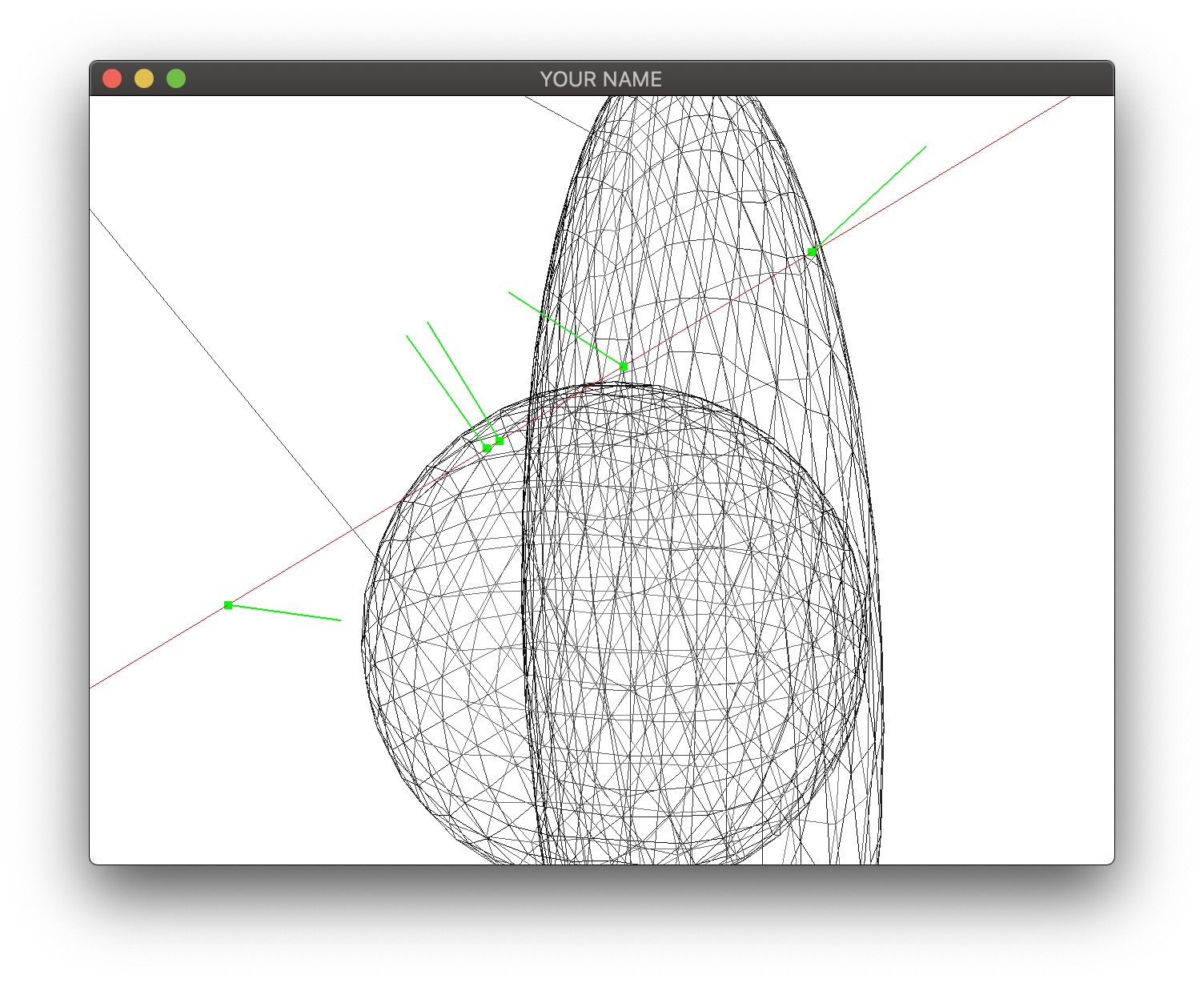
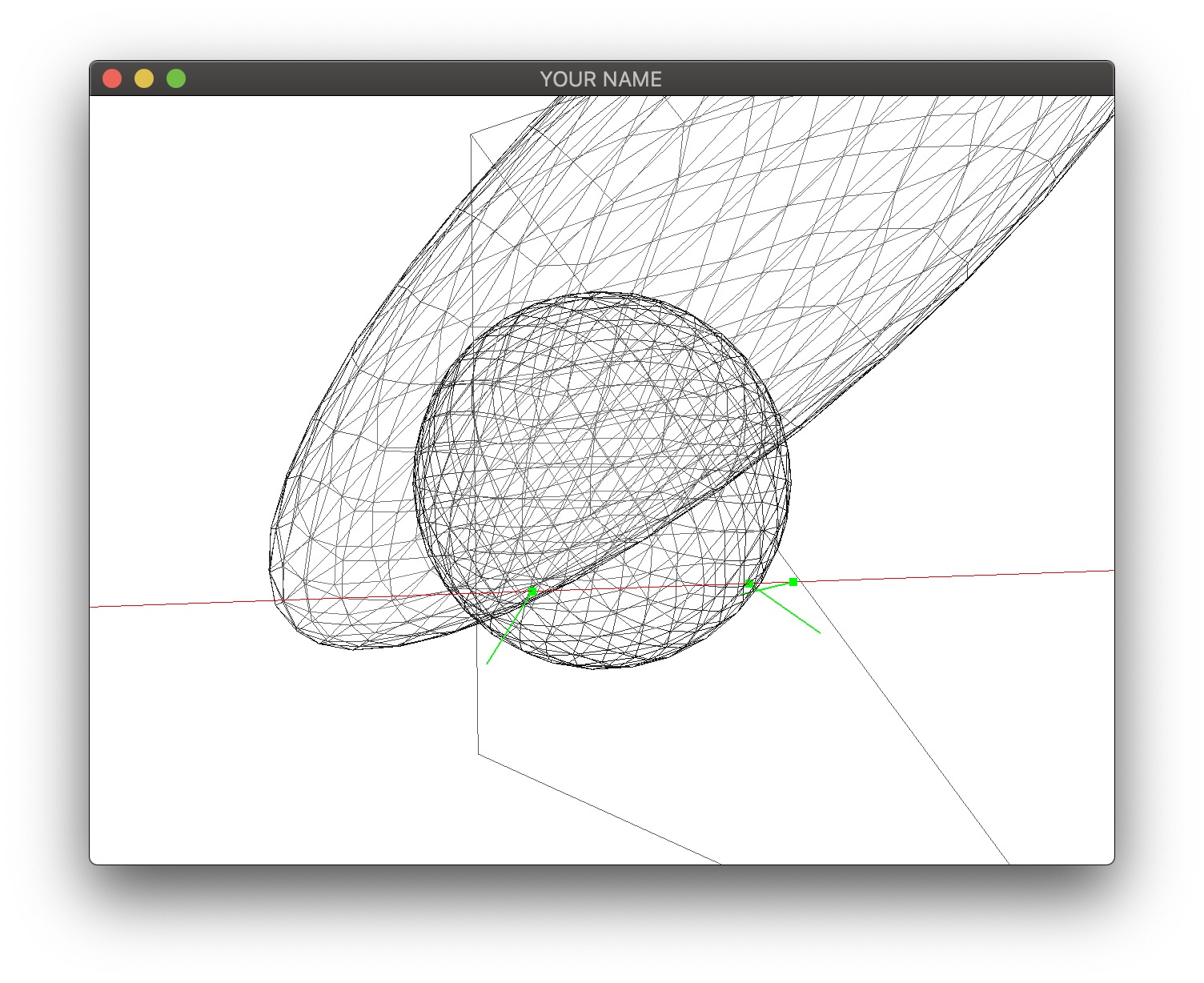
The z key toggles the wireframe mode, which will be useful for debugging.

Task 1

The first task is to update the ray whenever the mouse is clicked. We want to store the ray origin in ray[0] and the ray direction in ray[1]. (We will be using the world coordinate system throughout this lab.) The projection, view, and camera matrices (P, V, and C, respectively) are already computed for you in the previous lines.

Using the camera matrix, the position of the camera in world coords, which we denote \(\vec{c}_w\), is straightforward to obtain: it is simply the last column of the camera matrix. Store this in ray[0].

To get the ray direction, we need to go through the following series of transformations: pixel coords → normalized device coords → clip coords → eye coords → world coords. This is the reverse of the standard transformation for drawing things on the screen, and is described very nicely at http://antongerdelan.net/opengl/raycasting.html.

• Pixel coords → normalized device coords: To do this, you need to multiply by the inverse of the viewport matrix. However, rather than creating a matrix and inverting it, you can use the following: \[ \vec{p}_n = \begin{pmatrix} x_n\\ y_n \end{pmatrix}, \quad x_n = \frac{2 x_p}{width} - 1, \quad y_n = 1 - \frac{2 y_p}{height}. \] Here, the subscript \(n\) indicates normalized device coordinates, and the subscript \(p\) indicates pixel coordinates. Width and height are the x and y extents of the window. Note that the screen coordinate system inverts the y-axis so that the origin is at the top left instead of the bottom left. We do not need z here since any z-coord away from the camera can be used to compute the ray direction in normalized device coords.
• Normalized device coords → clip coords: To reverse the divide by w step (perspective division), we simply need to append \(-1\) to z and the usual \(1\) to w: \[ \vec{p}_c = \begin{pmatrix} x_n\\ y_n\\ -1\\ 1 \end{pmatrix}. \] It doesn’t matter what we put into w, so we put \(1\). We put \(-1\) in z, since we want the ray to point forward from the camera.
• Clip coords → eye coords: For this step, we use the inverse of the projection matrix: \[ \vec{p}_e = P^{-1} \vec{p}_c. \] Since this projection matrix affects the homogeneous coordinate, after this multiplication manually set the w component of \(\vec{p}_e\) to \(1.0\).
• Eye coords → world coords: For this step, we use the camera matrix (which is the inverse of the view matrix): \[ \vec{p}_w = C \vec{p}_e. \]

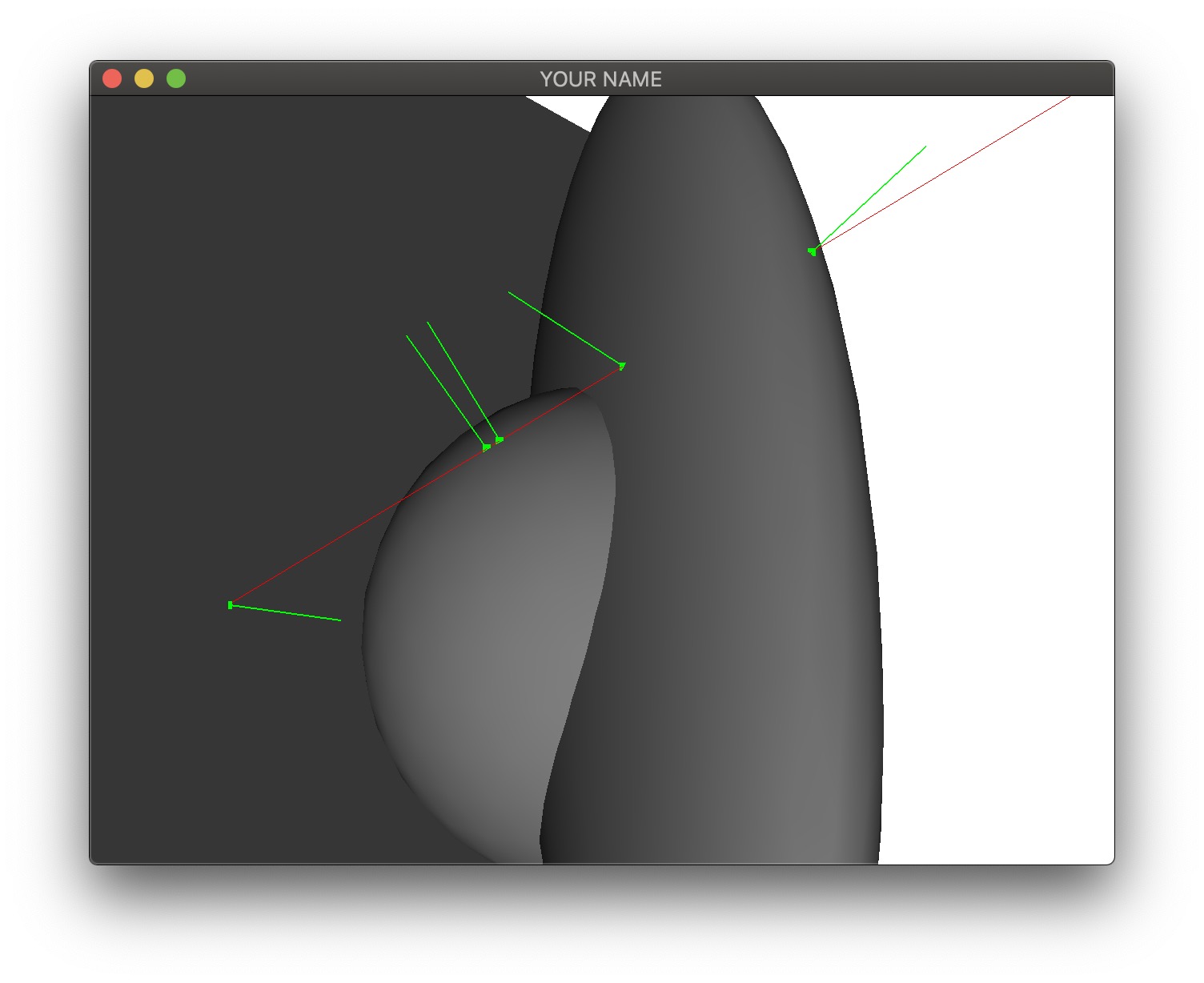
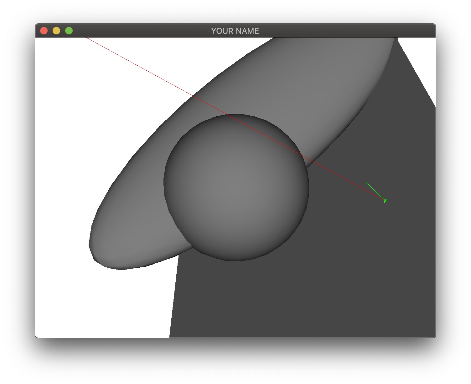
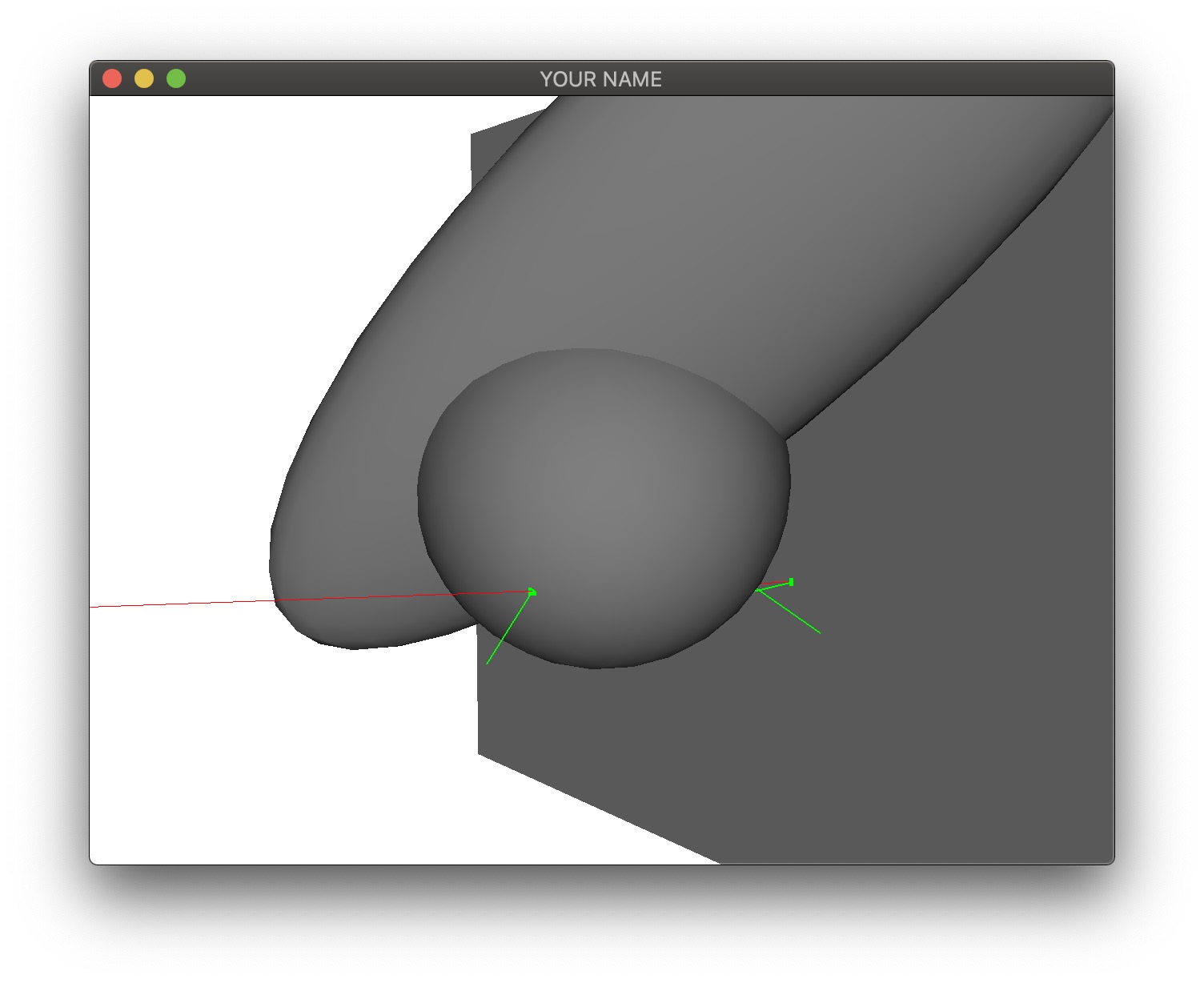
After all of these steps, we have \(\vec{p}_w\), a point whose position falls under the mouse in world coordinates. Note, however, that there are infinitely many such positions in 3D. What we’re interested in is the ray direction, so we subtract the camera position from this and normalize: \[ \hat{v}_w = \frac{\vec{p}_w - \vec{c}_w}{\| \vec{p}_w - \vec{c}_w \|}. \] Store this in ray[1]. Once \(\vec{p}_w\) and \(\hat{v}_w\) are correctly computed and stored, you should be able to shift-click on the window, rotate the view, and see the ray in red. In the video below, we are also visualizing the hit points in green, which will be implemented in the next tasks.

From this point on, we will drop the subscript \(w\) and assume that everything is in world coordinates.

Task 2

The next task is to compute the ray-plane intersection. We will assume that the plane is defined by a position \(\vec{c}\) and a normal \(\hat{n}\). For this lab, use the following: \[ \vec{c} = \begin{pmatrix}0\\0\\-1\end{pmatrix}, \quad \hat{n} = \begin{pmatrix}0\\0\\1\end{pmatrix}. \] Given the ray defined by \(\vec{p}\) and \(\hat{v}\), the intersection point, \(\vec{x}\), can be computed as: \[ t = \frac{\hat{n} \cdot (\vec{c} - \vec{p})}{\hat{n} \cdot \hat{v}}, \quad \vec{x} = \vec{p} + t \hat{v}, \] where \(t\) is the distance of the intersection point from the camera. Store \(\vec{x}\) and \(\hat{n}\) into a Hit object and add it to the hits vector. You should be able to see the hit point and normal in green.

Task 3

The next task is to compute the ray-sphere intersection(s). For this task, we will assume that the sphere is centered at the origin and has a unit radius.

First, we compute the discriminant of the quadratic formula using the ray origin and direction (\(\vec{p}\) and \(\hat{v}\)): \[ a = \hat{v} \cdot \hat{v}, \quad b = 2 (\hat{v} \cdot \vec{p}), \quad c = \vec{p} \cdot \vec{p} - 1, \quad d = b^2 - 4ac. \] If \(d < 0\), there are no intersections, if \(d = 0\), there is one intersection, and if \(d > 0\), there are two intersections. Due to floating point error, we can assume that there are either zero or two. If \(d > 0\), then the two hits are at: \[ t = \frac{-b \pm \sqrt{d}}{2a}, \quad \vec{x} = \vec{p} + t \hat{v}. \] For a unit sphere at the origin, the normal is the same as the position: \(\hat{n} = \vec{x}\).

Task 4

Next we are going to scale and translate the sphere. The sphere now takes two parameters: radius \(r\) and center \(\vec{c}\).

Like in Task 3, we compute the discriminant of the quadratic formula first: \[ \vec{pc} = \vec{p} - \vec{c}, \quad a = \hat{v} \cdot \hat{v}, \quad b = 2 (\hat{v} \cdot \vec{pc}), \quad c = \vec{pc} \cdot \vec{pc} - 1, \quad d = b^2 - 4ac. \] As before, there could be \(0\), \(1\), or \(2\) intersections. The normal of the hit point is the normalized vector between the hit point and the center: \[ \hat{n} = \frac{\vec{x} - \vec{c}}{r}. \]

Task 5

The final task is to transform the sphere into an ellipse. We start with an untransformed unit sphere from Task 3 (not Task 4), and then we create an arbitrary ellipsoid by transform it with translation, rotation, and scale. In this lab, we use the following transformation with the matrix stack M:

auto M = make_shared<MatrixStack>();
M->translate(0.5f, 1.0f, 0.0f);
glm::vec3 axis = normalize(glm::vec3(1.0f, 1.0f, 1.0f));
M->rotate(1.0f, axis);
M->scale(3.0f, 1.0f, 0.5f);
glm::mat4 E = M->topMatrix();

In other words, the sphere is transformed into the ellipsoid by the product E=T*R*S, which has the following numerical values:

E =

    2.0806   -0.3326    0.3195    0.5000
    1.9172    0.6935   -0.1663    1.0000
   -0.9978    0.6391    0.3468         0
         0         0         0    1.0000

To compute the intersections, we transform the ray into the local space of the ellipsoid. Using a prime (\('\)) to denote local-space quantities, we have: \[ \displaylines{ \vec{p}' = E^{-1} \vec{p} \quad \text{// use $1$ for homogeneous coord}\\ \vec{v}' = E^{-1} \hat{v} \quad \text{// use $0$ for homogeneous coord}\\ \hat{v}' = \frac{\vec{v}'}{\| \vec{v}' \|}. \qquad \qquad \qquad \qquad \qquad \qquad \qquad \; \; } \] Once \(\vec{p}'\) and \(\hat{v}'\) are computed, you can plug them into the sphere intersection code from Task 3 to compute \(t'\) and \(\vec{x}'\): \[ \displaylines{ a = \hat{v}' \cdot \hat{v}', \quad b = 2 (\hat{v}' \cdot \vec{p}'), \quad c = \vec{p}' \cdot \vec{p}' - 1, \quad d = b^2 - 4ac, \\ t' = \frac{-b \pm \sqrt{d}}{2a}, \quad \vec{x}' = \vec{p}' + t' \hat{v}'. } \] As before, there could be \(0\), \(1\), or \(2\) intersections. Finally, we transform the hit position, normal, and distance into world coordinates: \[ \displaylines{ \vec{x} = E \vec{x}' \quad \text{// use $1$ for homogeneous coord} \quad \,\\ \vec{n} = E^{-\top} \vec{x}' \quad \text{// use $0$ for homogeneous coord}\\ \hat{n} = \frac{\vec{n}}{\| \vec{n} \|} \qquad \qquad \qquad \qquad \qquad \qquad \qquad \quad \;\\ t = \| \vec{x} - \vec{p} \|. \qquad \qquad \qquad \qquad \qquad \qquad \quad \; \, } \] The absolute value for computing \(t\) implies that the returned \(t\) is always positive, even if the ellipsoid is behind the ray. Therefore, once \(t\) is computed, you should check if \(\vec{x}\) is behind the ray: \[ \hat{v} \cdot (\vec{x} - \vec{p}) < 0. \] If this is true, then set \(t = -t\).