In this lab, we are going to create a spherical surface procedurally in C++ and apply a texture to it in GLSL.
Please download the code for the lab and go over the code.
In our past labs, we loaded the mesh from an .obj file, but in this lab, we will be creating our mesh procedurally by defining the vertex position, normal, texture coordinates, and the triangle indices.
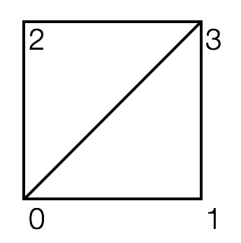
When you run the program initially, you’ll see a textured square. The camera can be controlled using the mouse. Study the function init() to understand how the vertex data are being specified. We are filling the position, normal, and texture coordinate buffers with data for the four vertices of the square. To create the two triangles that make up this square, we’re passing in 6 indices: 0 1 3 and 0 3 2. Press the ‘z’ key to toggle the drawing mode to wireframe to see the two triangles.
Note that the vertices are specified counter clockwise looking down the z-axis. This ordering implies that the “front side” of the triangle is facing the camera. If you press ‘c’, then OpenGL’s “cull face” mode will be turned on, making the “back side” of the triangles be invisible. With culling turned on, rotate the square 180 degrees to verify that it becomes invisible.
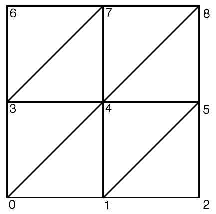
Remove the code for specifying the vertex data for the square and replace it with your own code that creates the triangulated grid shown below. Do not hard code anything. You should use a double for-loop; the outer for-loop should iterate over the rows, and the inner for-loop should iterate over the columns. (It may be helpful to do this in two stages: 1st double for-loop creates the vertices, and the 2nd double for-loop creates the triangle indices. There are other ways, of course.) The grid should be between -0.5 and 0.5 in both X and Y. The number of grid points in each direction should be a parameter (a local variable). In this figure, these numbers are 3 and 3, but make sure you can go up to at least 50 by 50. Since this grid lies on the X-Y plane, the normal is (0, 0, 1). To test if you have the vertices in counter-clockwise order, press the ‘c’ key to turn on/off back face culling. You should see the square from the front but not from the back.

Now we’re going to turn this grid into a sphere using spherical coordinates. In a spherical coordinate system, a point in 3D is defined using the radius (\(r\)) and two angles (\(\theta\), \(\phi\)).
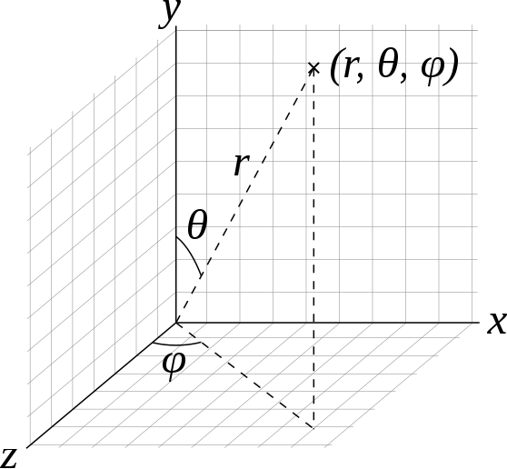
Spherical coordinates [Wikipedia]
For this lab, we will assume that the radius is constant: \(r=1\). So if we have \(\theta\) and \(\phi\), we can compute the corresponding 3D position, \(\vec{p}(\theta, \phi)\):
\[ \vec{p}(\theta, \phi) = \begin{pmatrix} \sin \theta \sin \phi\\ \cos \theta\\ \sin \theta \cos \phi \end{pmatrix}. \]
Note that the expression above isn’t exactly the same as the one in the Wikipedia article. This is because we are using the convention that Y is up.
How do we go about creating the vertex data for a sphere? In Task 1, we used a double for-loop to create a grid in the Cartesian space \((x,y)\):
for i = 1 ...
   for j = 1 ...
      x = ...
      y = ...
      z = 0
   end
end
Similarly, we can create a grid in the parametric space \((\theta, \phi)\). \(\theta\) should go from \(0\) to \(\pi\), and \(\phi\) should go from \(0\) to \(2\pi\).
for i = 1 ...
for j = 1 ...
theta = ...
phi = ...
x = sin(theta) * sin(phi)
y = cos(theta)
z = sin(theta) * cos(phi)
end
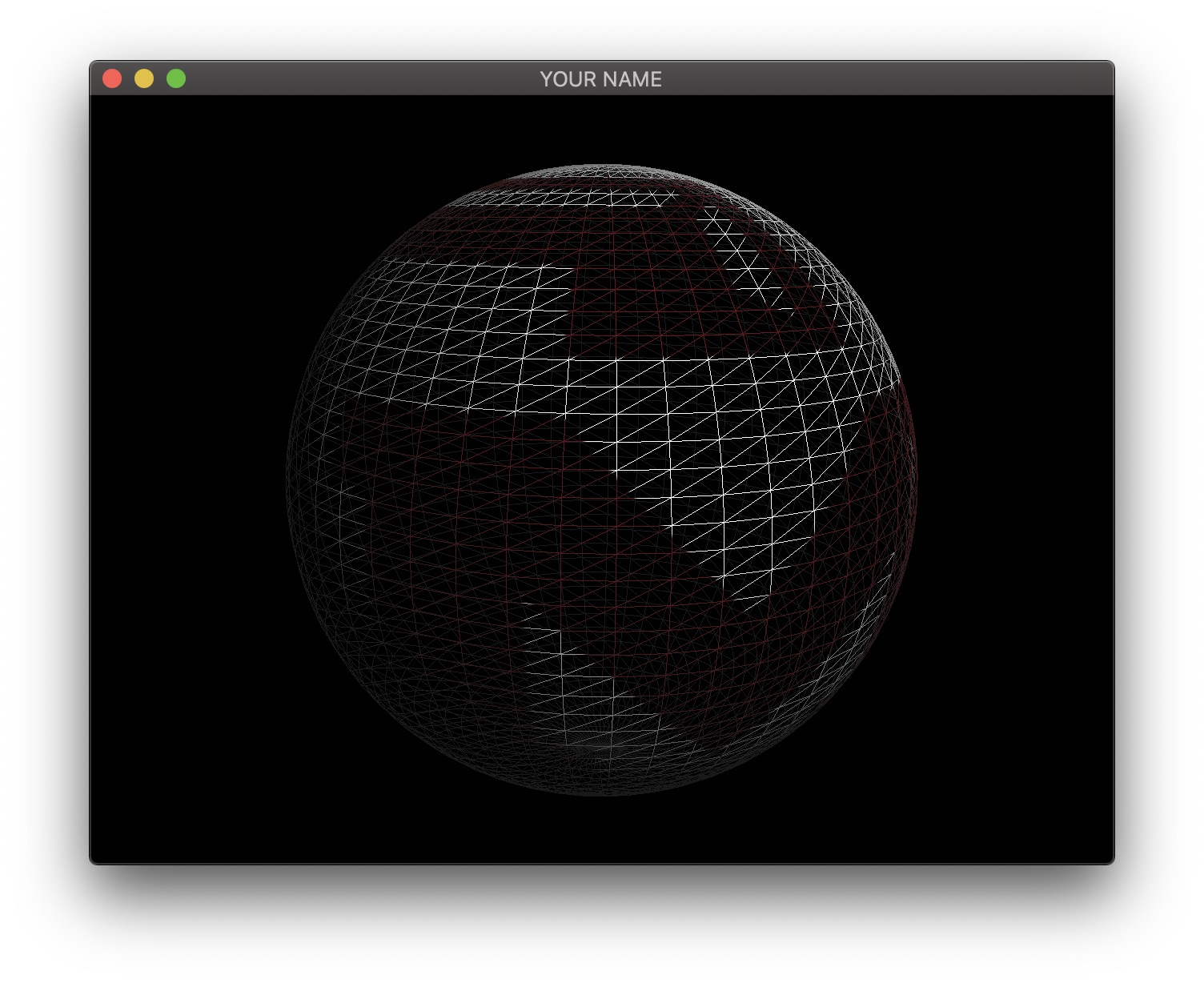
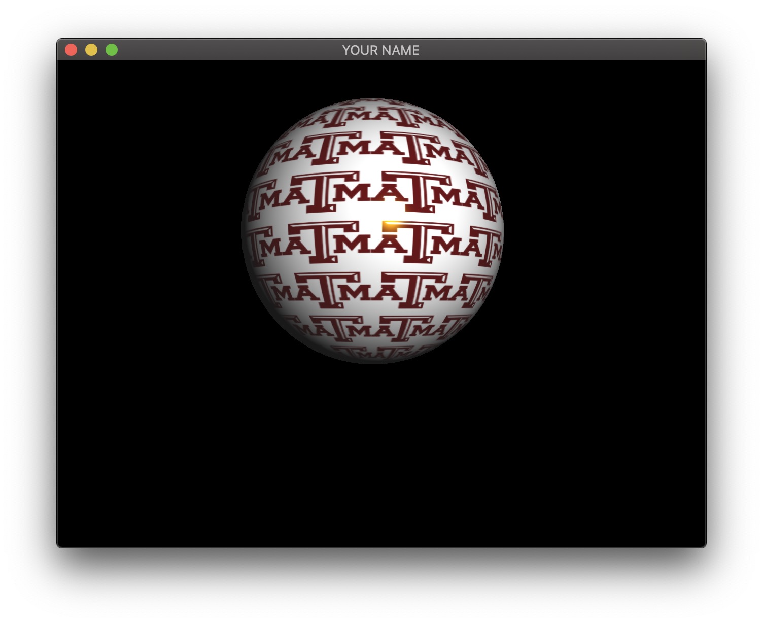
endFor a unit sphere at the origin, the normal is the same as the position. For texture coordinates, we can keep the same code from Task 1, which gives us the the Mercator projection. This will create a sphere with latitude and longitude lines, as shown below. The texture orientation will depend on how the texture coordinates were defined at each vertex. You may need to flip the y coordinate of the texture coordinate in the double for-loop. Optionally, you can further adjust the appearance of the texture by using a texture matrix.
Finally, we’re going to animate the sphere. We’re going to make it bounce up and down while changing the scale to “squash and stretch” the sphere.
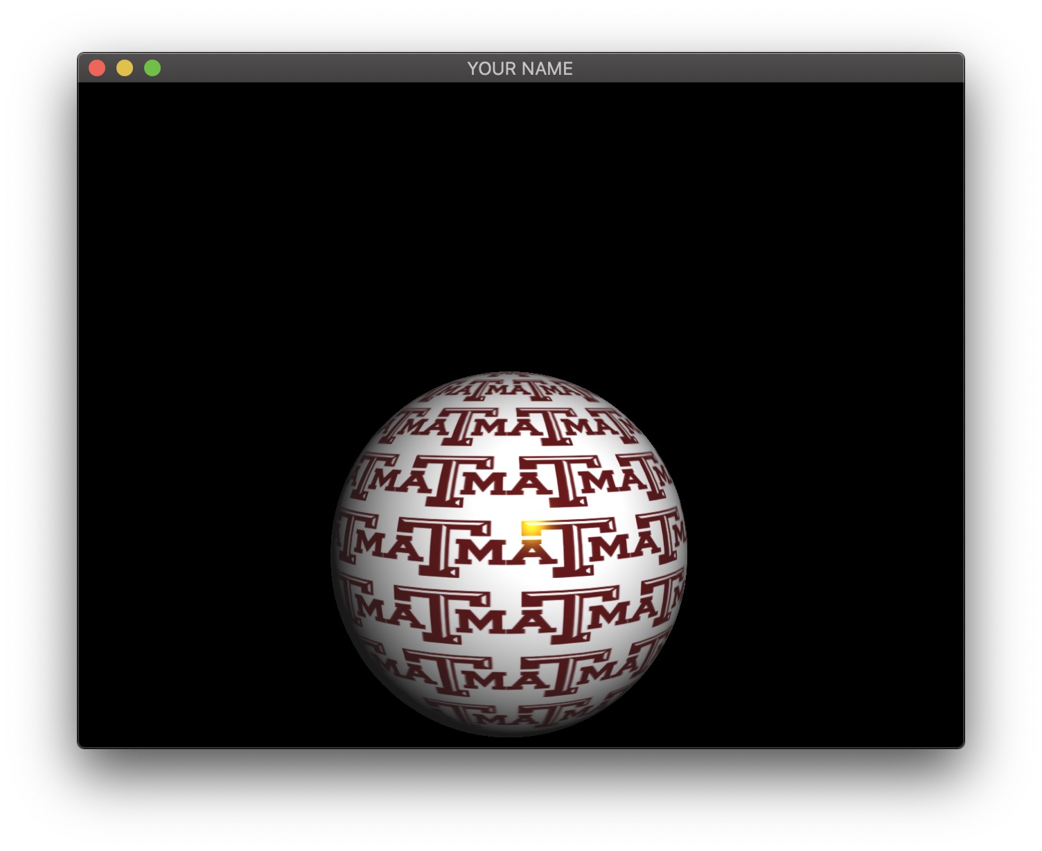
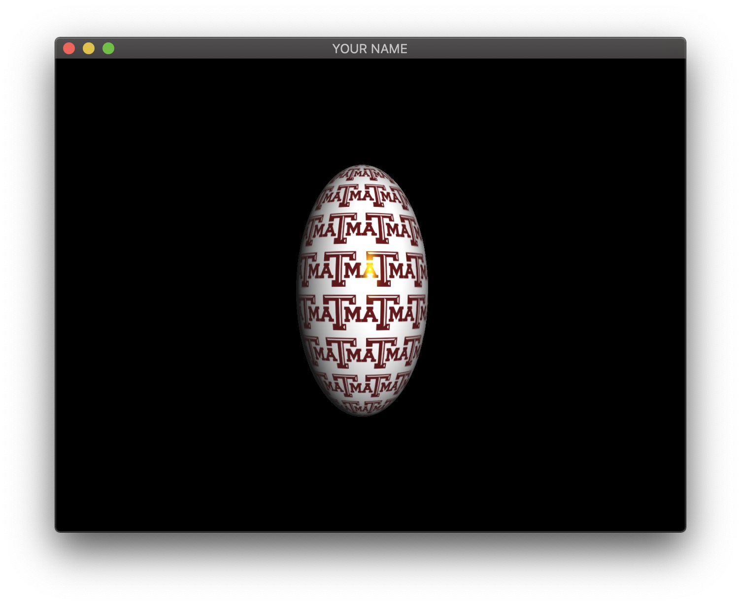
To do so, apply translation and scale to the modelview matrix. We want the Y translation to be a sinusoid with some amplitude, period, and phase. We also want the X and Z scale to be another sinusoid.
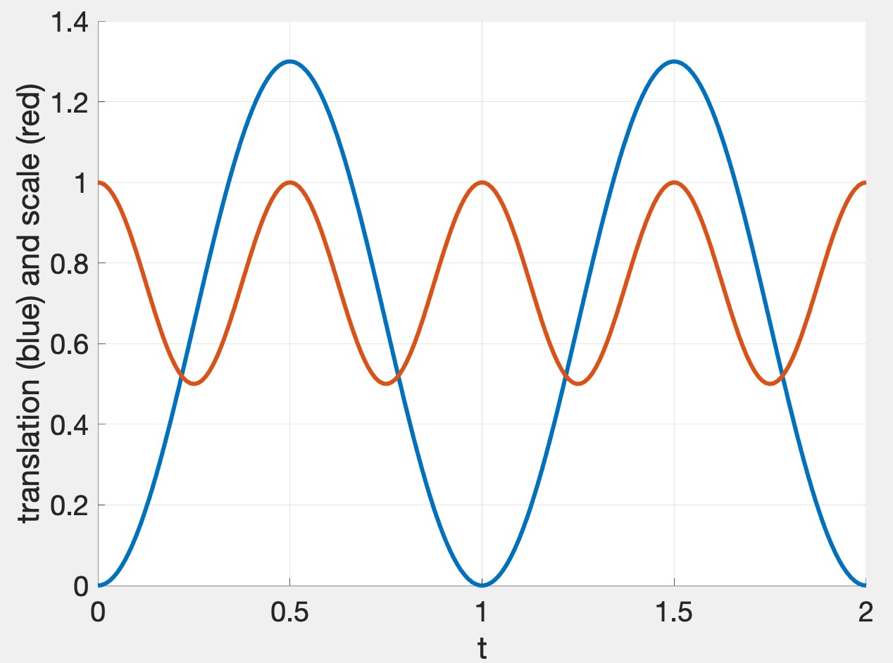
The graph above shows the translation in blue and scale in red. Since we want the sphere to bounce up, the blue curve has a minimum of \(0\) and a maximum of some height (\(1.3\) in this case). For squash and stretch, we want the sphere to get thinner while it is moving, so the red curve is twice as fast, with its peak value of \(1\) occurring when the sphere is stationary (at the low and high points of the blue curve). The functions that achieve this are:
\[ y = A_y \left( \frac{1}{2} \sin \left( \frac{2\pi}{p}(t + t_0) \right) + \frac{1}{2} \right)\\ s = -A_s \left( \frac{1}{2} \cos \left( \frac{4\pi}{p}(t + t_0) \right) + \frac{1}{2} \right) + 1, \]
where
Do not forget to send and use the inverse transpose of the modelview matrix in the vertex shader to transform the normal from model space to camera space. You need to multiply the incoming normal by the inverse transpose matrix and normalize the result.