1. Overview
This project was originally inspired by SPORE's procedural planet generation system. In particular, I used this image as my model. Some of the key aspects I wanted to implement were the following:
- Realtime generation of planet terrain and features (water, foliage)
- Cloud/atmosphere simulation/emulation
- Day/Night simulation (shadows, and a starry night sky)
- Water simulations for ocean and flowing rivers
In the end, I was able to accomplish a fairly decent approximation of the what SPORE does. I got a world to generate on-the-fly with atmosphere, ocean, texturing, a galactic backdrop. I even added my own little flair of plant-life to populate the surface of the world.
2. Process
2.1 Starting Point
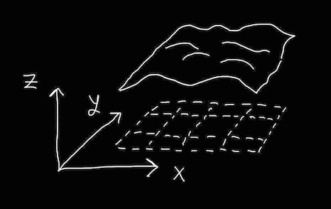
The algorithm for generating my height fields works by splitting up a rectangle into smaller, equally sized sections and then calculating the height for each rectangle to create an approximation of the height field, as shown in Figure 2.1.1. Each smaller rectangle can then be used to make two triangles (the approximated face) for the height field by adding the vertices counterclockwise.
Next, I needed to find the normal for each vertex. To do this, I sampled three points around each vertex and used them to find the normal for the triangle they formed, as shown in Figure 2.1.2. By taking the epsilon from the original vertex to be very small, I arrived at a very close approximation of the normal at each vertex.
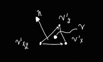
So:
h(x, y) = PerlinNoise(x, y)
e = 0.0001

v    = h(x, y);
v'xy = h(x - e, y - e)
v'x  = h(x + e, y)
v'y  = h(x, y + e)

n = crossProduct(v'x - v'xy, v'y - v'xy)
For texture coordinates, I map each mini-rectangle to the (1, 0) x (0, 1) texture map space based on which portion the particular vertex lies in the overall height field rectangle. In the final version, I made it so that for each vertex there is an X by Y number of pixels that are colored in the texture.
2.2 Cartesian Implementation
During previous projects for the course I slowly developed a library of functions, classes, and designs that ultimately made it so I could approximate what we see in SPORE in only 2-3 weeks. Specifically, in a previous assignment I had developed an algorithm for creating square height fields using Perlin noise, as shown in Figure 2.2.1.
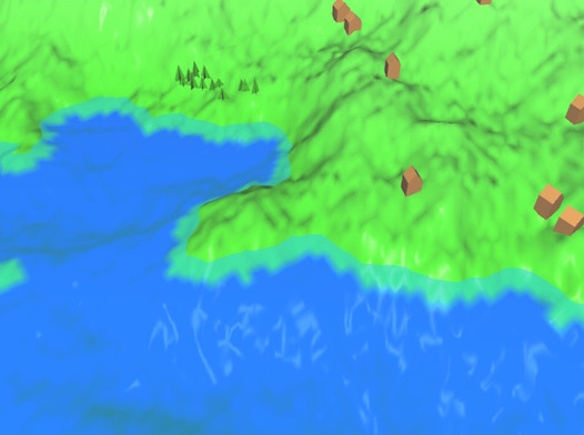
To generate the terrain, I used several octaves of Perlin noise to create a height field using the output as the z-value. I then filtered and accentuated the noise at specific intervals to modify the resulting heights in order to create a more distinguished landscape. Then I mapped a texture pixel to each vertex depending on the specific heights of where each vertex fell. For example, at a certain point I changed the color from blue ("ocean") to green ("land"). This, along with a slightly transparent "water surface", creates the illusion that we're looking at a landmass that is in a pool of water.
As the terrain generates (in a spiral around the origin), my generation functions gather sample points that are "above water". Intersecting these points with a differently seeded Perlin noise function, I get an effect where the trees are placed in curved blotches.
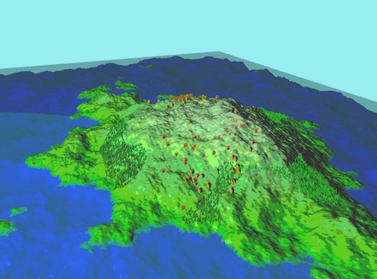
The reason I use a toon shader (distinct grades of color) is because the final result doesn't look very pretty. Changing the shader to a simple blinn-phong shader reveals that the texturing process is both (1) not high resolution enough and (2) needs more gradation (which is sort of achieved using the toon shader) as shown in Figure 2.2.2. Notice the jagged edges and strange dark lines on the terrain.
2.3 Spherical Implementation
With planet generation, I would need to change my algorithm from making a square, xy-plane height field, into a spherical height field system. From this, and the texturing issue mentioned above, these are the main problems I would need to address:
- Higher resolution texture mapping onto height field
- Better blending of texture colors on height field
- Building a Spherical height field
For generating spherical heightfields, all I have to do is change my perspective: xyz becomes theta, phi, and radius respectively. Then when I'm actually creating my sphere in in 3D space, I can convert each (radius, theta, phi) into the corresponding (x, y, z) (see Wolfram Alpha) so that my Perlin noise function and height field algorithm still works as intended. Note that if I take theta to go from 0 to 2 * pi and phi from 0 to pi, my height field algorithm with generate an entire sphere, as illustrated in Figure 2.3.1. This was useful for generating spheres for other parts of my project, as is discussed in Section 3.
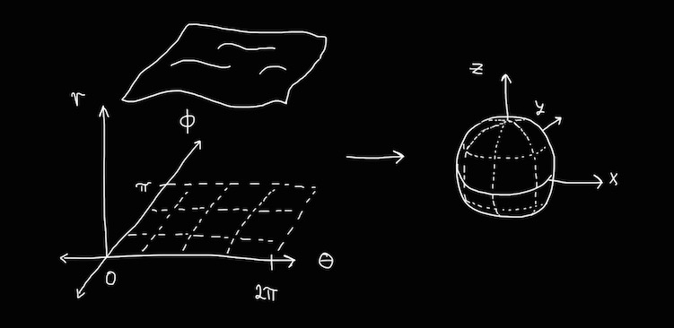
Here, the major issue (that I didn't have time to address) was that the polar caps have "smashed" in spherical rectangles (essentially a spherical triangle) rather than actual spherical rectangles. This crops up as a visual issue later in the project with texturing and leads to some interesting bugs with normal calculation and rendering the polar caps.
Bringing this all together results in a sphere where the surface is continuous but also nicely amorphous, as shown in Figure 2.3.2.
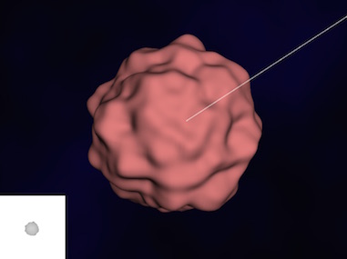
The white lines and the box in the bottom left are for debugging purposes and represent the clip-coordinate space for the light source and the result of creating a shadow map for the sphere.
3. Final Result
3.1 Terrain Texturing, Ocean, Atmosphere, and Galaxy Sky-box
The terrain for the sphere is largely colored the same way as in Figure 2.2.1, except I solve the issue of jagged rendering and blending by doing my own pre-blending when I'm building the sphere. In particular, each terrain (ocean, sand, savanna/rocks, greenland, mountain) has its own identifying color. Whenever the calculated radius exists between any two types of terrain, the resulting color is a proportional blend from one to the other. In addition, I employ addition noise around the edges to make transitions less uniform and have a more natural look to them.
Since I did not have enough time to make an ocean simulation, I stuck to doing something much simpler: I reused my spherical height field generator to look blue like the ocean, then recreated it about every draw frame to give the effect that the ocean's water is sloshing around over time.
For the atmosphere I focused on approximating the "faint glow" around the edges. I did this by placing a semi-transparent sphere around my world and then wrote a shader that computes the alpha value for each fragment to be less if the reflected eye vector on that point was more "glancing". The result is a faint haze around the world.
Around the world exists a "galactic" sky box which emulates the stars in the night sky and even arms of the Milky Way. I did this by reversing the direction that my spherical height field algorithm runs, so instead of making phi go from 0 to pi, it instead goes from pi to 0. The result is the the texture is mapped inside the sphere. Then I blend a few faint colors against the Perlin nosie function, and sample hundreds of points to place "stars" in the texture.
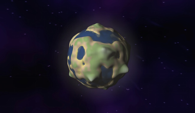
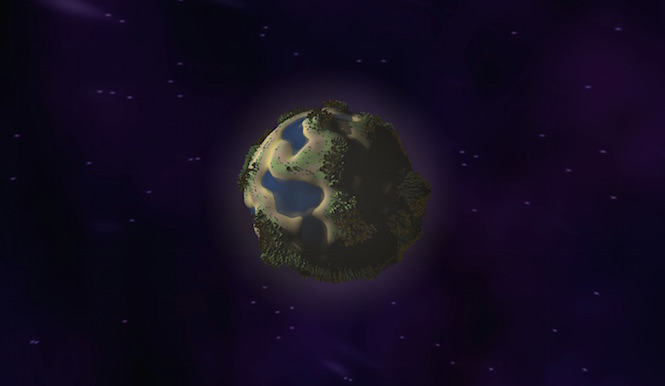
The result of a blended terrain, the emulated ocean, the atmosphere shader, and the galactic skybox (as well as tinkering with how the radius is generated) is a fairly good-looking "tiny" planet, as shown in Figure 3.1.1.
3.2 Fauna
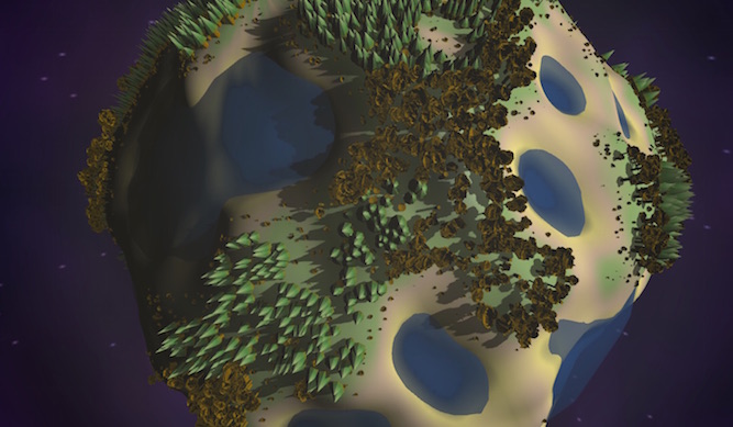
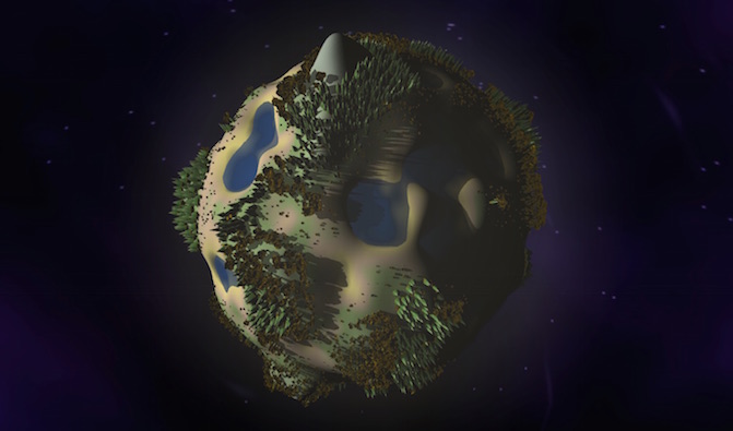
For plant-life, I used a similar technique as described in section 2.2 for placing various kinds of plants. I had four kinds of plants (pine trees, bushes, "bushy trees", and tree stumps), each of which I generated on-the-fly by using Perlin noise in combination with arc4Random to determine the height and radius of each. By using the intersection of two Perlin noise functions, I was able to get an effect where trees tend occur in groups that touch one another, as shown in figure 3.2.1.
3.3 Project In Action
The final product that I presented in class is shown in Figure 3.3.1 and Figure 3.3.2. When the project starts up the screen is completely black, and over time the world and skybox build incrementally over the next 15 seconds.
The project has a few controls:
Keyboard Controls:

 Camera:
   WASD  - move camera relative to planet (buggy).
   QE    - move farther/closer to the planet.

 Planet:
   P     - "pause" the application (building and rotation of planet)
   R     - toggles the rotation speed from slow to slightly faster

 Mouse:
   C     - toggles whether the mouse is "captured" in the window.
   H     - toggles whether the mouse is hidden from view.

 Misc:
   L     - toggles whether shapes are drawn using "lines" or "faces"
The following is a live demo of the project on YouTube:
3.4 Unresolved Issues
The largest constraint for this project was time: I didn't have time to figure out simulations, and I didn't have time to improve some of my generation algorithms. It is for this reason that I didn't end up implementing clouds because as a particle system it didn't work very well (texturing was buggy, and the physics was hard to get right) and when looking through academic papers, the implementation of a more realistic simulation seemed beyond what I could do in 2.5 weeks.
Other issues include that the polar caps of spheres didn't equally map textures to the surface. This was inherent because when creating a polar cap, the bottom edge of the "theta axis" smashes into a single point in cartesian coordinates. This means that the edges of the texture are now crammed into twice the space than everywhere else on the sphere. This lead me to hiding away the poles as much as possible from view. In the video if you pay attention to the north pole of the planet that the water is a little darker and has radial lines. This is the effect of this bug in my height field algorithm. Additionally, I took to creating lower resolution polar caps so the texture cramming issue wasn't as apparent.
If you demo the project, when you look at the south pole you'll see a "hole in the ozone". This was a bug I could not figure out for the life of me.
4. Resources and References
Important Links:
- Project Demo YouTube Video
Primary Sources:
- This project made extensive use of glm
- I used and modified a Perlin Noise C++ class available online from sol-prog
- Shinjiro Sueda for lots of sample code and advice.
- I used tinyobjloader for testing and building shapes on-the-fly.
- This application is built on OpenGL and GLUT
Other sources:
- Tips for using GLUT and warping the mouse pointer
- Wolfram Alpha for spherical coordinate conversions
- Zoe Wood for GLSL helper functions