OpenGL Game of Life
- Created by
- Drew Troxell
- Class
- CPE 471
- Professor
- Dr. Shinjiro Sueda
- Based on
- Conway's Game of Life
OpenGL Game of Life is a cellular automation simulation based on the famous Conway's Game of Life. This implementation of the simulation is meant to expand the simulation into a 3 dimensional object space and allow for users to view the cellular automation in a 3D environment. Other 3D implementations of Conway's Game of Life exist, but these implementations modify the game rules to work with a 3 dimensional array of cells. This implementation of the game of life uses the traditional 2 dimensional array of cells for the automation, but includes extra rules to modify the shape of the cells to simulate the growth of population centers over time.
Download
Download OpenGL Game of Life for OSXTechnical Details
Rules of the Game
Conway's Game of Life is based on four very simple rules applying to a 2x2 array of cells. Each cell can have one of two states: alive or dead. Each state change of the game occurs simultaneously accross all cells and is called a "tick." The rules to determine the state change of cells between ticks is as follows:
- Any live cell with fewer than two live neighbours dies, as if caused by under-population.
- Any live cell with two or three live neighbours lives on to the next generation.
- Any live cell with more than three live neighbours dies, as if by overcrowding.
- Any dead cell with exactly three live neighbours becomes a live cell, as if by reproduction.
The OpenGL Game of Life operates under the same set of rules as Conway's Game of Life to determine the next state of individual cells. All cell state calculations occur simultaneously as well. The only difference in the rules between this implementation and the traditional implementation are for cells that continue on to the next generation. Any cell that lives to another generation will slightly increase in size. This allows the 3D game of life to simulate the rise of large cities and population centers in 3 dimensions. The overall rules of OpenGL Game of Life are as follows:
- Any live cell with fewer than two live neighbours dies, as if caused by under-population.
- Any live cell with two or three live neighbours lives on to the next generation. The size of the cell increases in height by 0.4 and in width by 0.05.
- Any live cell with more than three live neighbours dies, as if by overcrowding.
- Any dead cell with exactly three live neighbours becomes a live cell, as if by repr oduction.
Initial Seeding
The game begins with a pseudorandom collection of alive and dead cells spanning the size of the array. Macros exist to modify the amount of the array to initialize and the overall size of the array. The random selection of cells to initialize as alive or dead is based on seeding against the time of the machine since system epoch. Each cell checks against rand() % 2 to determine whether it should initialize as living or dead.
Color Coding of Buildings
OpenGL Game of Life includes materials for three different types of building: residential, commercial, and industrial. When the game begins, all living cells are residential (light brown). This is to reflect the initial state of fledgling communities as largely residential. Any cells that live on between generations, however, can take on a new color, which is a pseudorandom selection between commercial (yellow) and industrial (dark brown). Any dead cell that becomes alive always starts as a minimum size residential material object.
Optimization for Large Datasets
One of my main goals in creating OpenGL Game of Life was to be able to simulate massive populations of cells in 3 dimensions. In my initial implementation of the game, the handling of each object within the various cells and the calculations to determine the next state for each cell limited my cell array size to 12x12 before leading to crashing and bugs. Only 144 cells was far too low to achieve the scale that OpenGL Game of Life needed to be a real interesting simulation of population centers. Two improvements have since allowed for datasets of as much as 500x500 or even more! The first is using a single object for all cells, and the second is the use of threading to computer cell next states.
In order to improve loading times for game start up and minimize the amount of information being processed multiple times unnecessarily, the first optimization to the game was creating a single object for all cells to draw. Initially, each cell held a copy of an object to be drawn. This meant that each cell had to initialize and load its object before the game could begin. It also meant that each cell held a copy of a large data structure for the object, leading to memory issues at large datasets. To eliminate this, a single object was created to represent the object drawn within a cell. Each cell then holds a pointer to this object, allowing all cells to run with only a single object as overhead.
The improvement to the object allocation improved loading times and the size of the dataset which could be drawn, but did not help with the processing of state changes. In order to calculate the next state of each cell, the program must loop through every cell in the 2x2 array, and then for each cell it finds it must loop through a 2x2 array of the cells neighboring that cell. This leads to performance of O(n^2 * m^2), where n is the length of a side of the 2x2 array of cells and m is the length of a side of the 2x2 array of neighbors. In order to eliminate the strain this computation placed on the drawing section of the code, the code to determine the next state of each cell was placed in a separate function. This function is run on a separate thread from the main game, allowing for the computation of the next states to run independently from the drawing of each cell. This allows for massive sets of data to be computed without slowing down the runtime of the graphics in the simulation.
Pictures
Photos with captions.
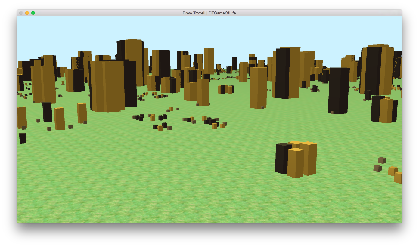
Early stages of cellular automation. Distinct communities beginning to form.
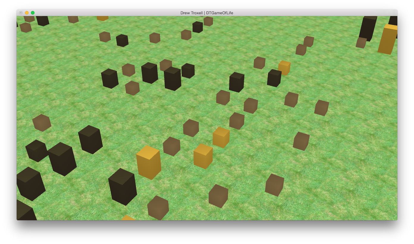
Close-up showing the different types of buildings.
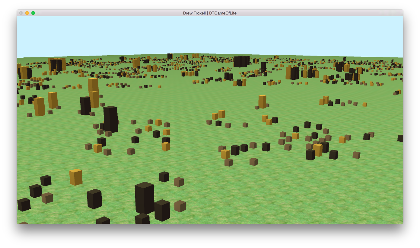
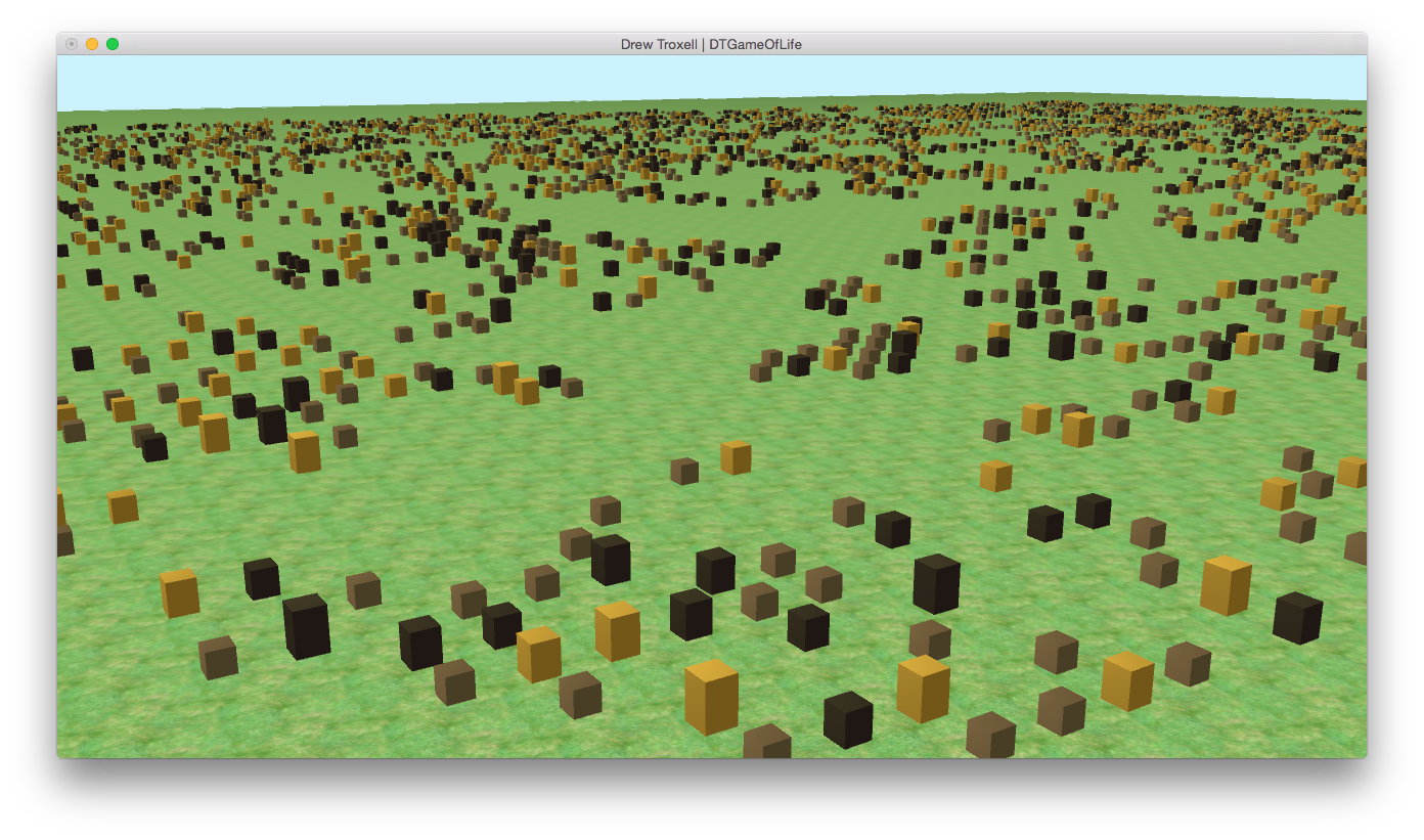
Showing most of the population of the 300x300 simulation after enough iterations to begin forming large structures.
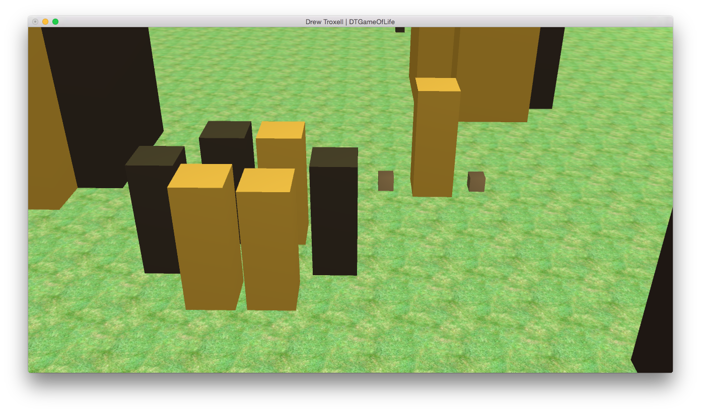
Close-up of two common stable states in the cellular automation.
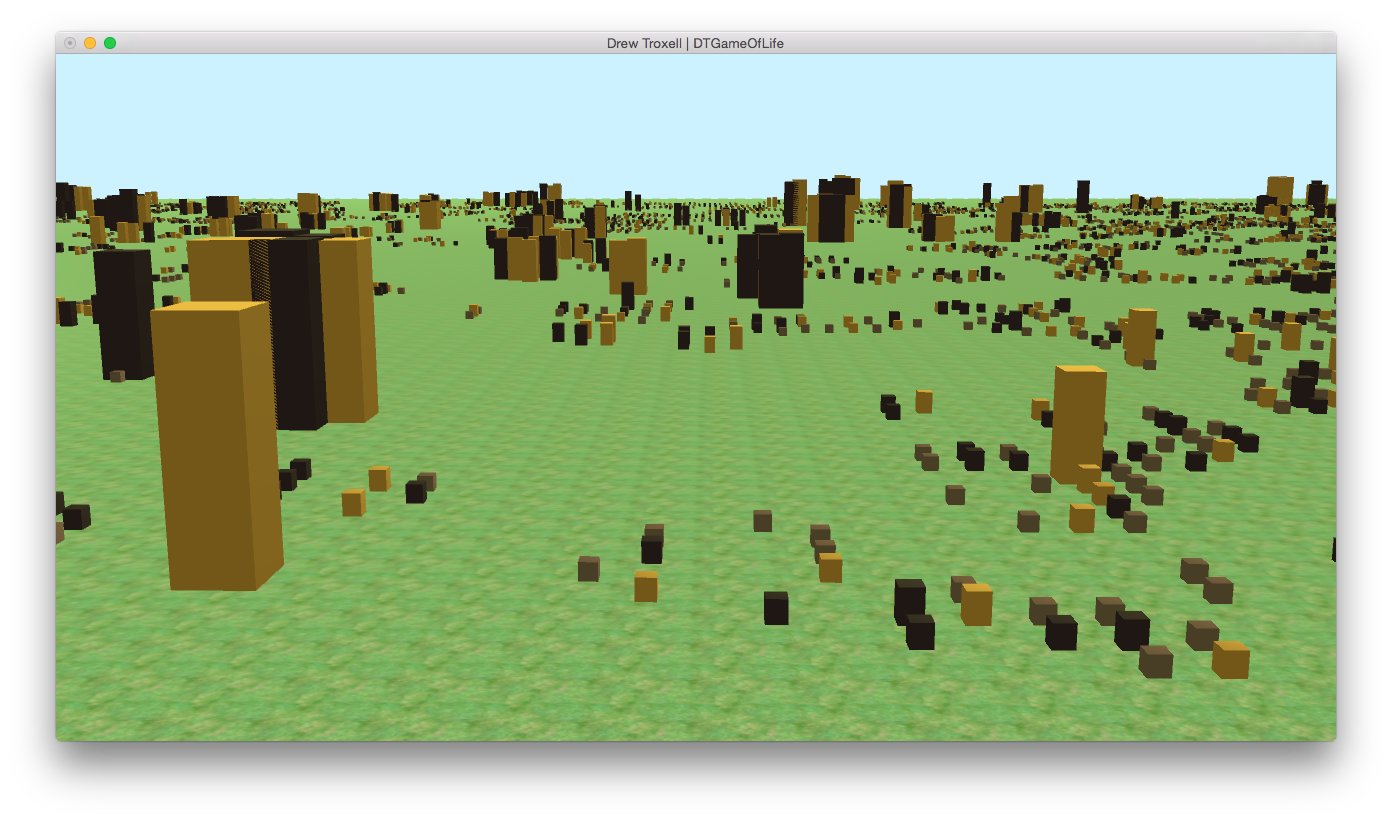
Wide screenshot of the simulation after enough iterations for a distinct skyline.
A screenshot after only a handful of iterations. This is close to what an initial seed looks like.
Video
Demo of a 300x300 cell simulation.
Resources
The following are resources I either used or found helpful in the course of developing OpenGL Game of Life:
- Open Game Art - A good resource for free graphics assets.
- Wikipedia Conway's Game of Life - Provides background on the cellular automation rules.
- r/gamedev - An excellent community of aspiring game developers.
- Foundations of Computer Graphics by Steven Gortler - The class text is an excellent resource for OpenGL basics.
Future Work
My ambitions for this project were much larger than what I was able to accomplish over the course of the last couple of weeks of classes. That being said, I am extremely happy with the result. Here are a few improvements I hope to make in the future:
- Height Field Terrain
- Instead of using a flat surface, create a height field based pseudo random terrain and include it as part of the rules of life. For example, cells on steep slopes cannot be alive cells due to the terrain. It would be interesting to see how the automation handles the terrain limits rather than an open 2x2 grid.
- Textured Buildings
- While the materials currently in the game are nice and allow for the distinguishing between different buildings by color, using actual textures for the buildings would be an improvement visually for the game. Applying a texture to represent a residential building, a commercial building, and an industrial building would add some visual appeal to the automation.
- Day/Night Cycle
- Having a day/night cycle would improve the visuals of the game and lend itself to the concept of populations changing over time.
- Shadow Mapping
- Along with a day/night cycle, shadow mapping would providing tasty visuals for those watching the simulation.