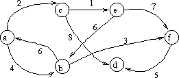
Consider a weighted, directed graph
G = (V, E, w).
V is the set of vertices.
E is the set of edges that are order pairs linking the vertices.
w is a function from E to the real numbers
giving the weight of an edge.
For example, in the following graph:

A weighted graph can be represented as an adjacency matrix whose elements are floats containing infinity (or a very large number) when there is no edge and the weight of the edge when there is an edge. Adjacency lists can also be used by letting the weight be another field in the adjacency list nodes.
In the algorithm, we will arrange V as an sequence from 1..n, with vertex #1 being the source vertex. We'll have an array D[2..n] keeping track of the current minimum distances; at any point in the algorithm, D[i] is the current minimum length of a path from vertex #1 to vertex #i. There is a priority queue Q that contains vertices whose priorities are their values in D (smaller value means higher priority, as with Huffman's Algorithm). Note that the priority queue must be able to automatically account for adjustments to D, so we'll have to adjust the queue each time through a loop. This is pseudocode for the algorithm:
Dÿkstra (G, s) {
	n = |V|
	for (i=2; i<=n; i++) {	// initially, D[i] is the weight
		D[i] = w (1, i)		// of the edge from vertex 1 to i,
	}				// which might be infinite
	for all i >= 2 in V, insert i into Q, using D[i] as the priority
	for (i=0; i<=n-2; i++) {
		v = Extract-Minimum (Q)	// v is the closest vertex to #1
		for each vertex w left in Q {
			D[w] = min (D[w], D[v] + w (v, w))
		}
	}
	return D
}
D starts out as the obvious first guess: the length of the
edge from 1 to i for i in 2..n. This might
not be the best guess, especially if there is no edge and the w
function returns infinity. Q starts with all the vertices in
it.
In a loop, we go toward the vertex v closest to 1, the minimum element in the queue. At this point, we know the length of the minimum path from 1 to v that doesn't go through any of the vertices in Q. We then update D, offering each other vertex w a possibly shorter path length from vertex 1 via v, i.e., path from 1 --> v --> w. If the length in D is greater than this length, we replace it.
At the end of the algorithm, all vertices but the farthest one from 1 have been removed from the queue, thus D has the lengths of the shortest paths through any vertex.
Let's use the above graph for an example of Dÿkstra's Algorithm starting from vertex a:
Initially:
Q = { b, c, d, e, f} (think of them as 2..5)
	    b  c  d  e  f
D[2..5] = [ 4  2 oo oo oo ]

repeat loop starts:

minimum v from Q = c, with D[c] = 2.  Now Q = { b, d, e, f }.
Look at path lengths from a through c to { b, d, e, f }
	D[b] = 4,  D[c] + w (c, b) = oo, no change.
	D[d] = oo, D[c] + w (c, d) = 8, so now D[d] = 8 (a->c->d)
	D[e] = oo, D[c] + w (c, e) = 3, so now D[e] = 3 (a->c->e)
	D[f] = oo, D[c] + w (c, f) = oo, no change

          b  c  d  e  f
Now D = [ 4  2  8  3 oo ]

minimum v from Q = e, with D[e] = 3.  Now Q = { b, d, f }
Look at path lengths from a through e to {b, d, f}
	D[b] = 4, D[e] + w (e, b) = 9, so no change.
	D[d] = 8, D[e] + w (e, d) = oo, so no change
	D[f] = oo, D[e] + w (e, f) = 10, D[f] = 10 (a->c->e->f)

          b  c  d  e  f
Now D = [ 4  2  8  3 10 ]

minimum v from Q = b, with D[b] = 4.  Now Q = { d, f }
Look at path lengths from a through b to {d, f}
	D[d] = 8, D[b] + w (b, d) = oo, so no change.
	D[f] = 10, D[b] + w (b, f) = 7, so D[f] = 9 (a->b->f)

          b  c  d  e  f
Now D = [ 4  2  8  3  9 ]

minimum v from Q = d, with D[d] = 8.  Now Q = { f }
Look at path length from a through b to f
	D[f] = 9, D[d] + w (d, f) = oo, so no change.

We are done; f is the only element of the queue, so it can't help make
any other path lengths shorter.

      b  c  d  e  f
D = [ 4  2  8  3  9 ]
If we assume an
adjacency matrix representation, then w is just an O(1)
array access and Q is a queue of array indices. Storage
for an adjacency matrix is
 (n2).
If we know that there are very few edges, an adjacency list representation
would be more appropriate. We'll assume a matrix representation for the
analysis.
If we want to use a heap-based priority queue, we'll have to call Heapify each time D is updated, which happens O(|Q|) times throughout the repeat loop and takes O(ln |Q|) time for each call.
The initialization of D is
 (n), the
initialization of the queue is O(n ln n)
(n inserts into a heap, each costing O(ln n) time).
The for (i=0; i<=n-2; i++) loop happens n-2 times. Let e = |E|, i.e., the number of edges. No edge is considered more than once in the for each edge loop, so this is an upper bound on the number of possible updates to D and thus calls to Heapify, which each cost O(ln n) time. We must do an Extract-Minimum each time through the for (i=0; i<=n-2; i++) loop, each of which also cost O(ln n) time. So we the algorithm runs in time O(n ln n) (for initializing the queue) + O(n ln n) (for the calls to Extract-Minimum) + O(e ln n) (for all the calls to Heapify when we update D), = max (O(n ln n), O(e ln n)).
The name "transitive closure" means this:
We'll represent graphs using an adjacency matrix of Boolean values. We'll call the matrix for our graph G t(0), so that t(0)[i,j] = True if there is an edge from vertex i to vertex j OR if i=j, False otherwise. (This last bit is an important detail; even though, with standard definitions of graphs, there is never an edge from a vertex to itself, there is a path, of length 0, from a vertex to itself.)
Let n be the size of V. For k in 0..n, let t(k) be an adjacency matrix such that, if there is a path in G from any vertex i to any other vertex j going only through vertices in { 1, 2,..., k }, then t(k)[i,j] = True, False otherwise.
This set { 1, 2, ..., k } contains the intermediate vertices along the path from one vertex to another. This set is empty when k=0, so our previous definition of t(0) is still valid.
When k=n, this is the set of all vertices, so t(n)[i,j] is True if and only if there is a path from i to j through any vertex. Thus t(n) is the adjacency matrix for the transitive closure of G.
Now all we need is a way to get from t(0), the original graph, to t(n), the transitive closure. Consider the following rule for doing so in steps, for k >= 1:
t(k)[i,j] = t(k-1)[i,j] OR (t(k-1)[i,k] AND t(k-1)[k,j])In English, this says t(k) should show a path from i to j if
Warshall (G) {
	n = |V|
	t(0) = the adjacency matrix for G

	// there is always an empty path from a vertex to itself,
	// make sure the adjacency matrix reflects this

	for (i=1; i<=n; i++) {
		t(0)[i,i] = True
	}

	// step through the t(k)'s

	for (k=1; i<=n; k++) {
		for (i=1; i<=n; i++) {
			for (j=1; j<=n; j++) {
				t(k)[i,j] = t(k-1)[i,j] ||
					(t(k-1)[i,k] && t(k-1)[k,j])
			}
		}
	}
	return t(n)
}
This algorithm simply applies the rule n times, each time
considering a new vertex through which possible paths may go. At the
end, all paths have been discovered.
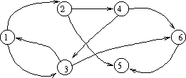
Let's look at an example of this algorithm. Consider the following graph:

So we have V = { 1, 2, 3, 4, 5, 6 } and E = { (1, 2), (1, 3), (2, 4), (2, 5), (3, 1), (3, 6), (4, 6), (4, 3), (6, 5) }. Here is the adjacency matrix and corresponding t(0):
down = "from"
across = "to"

adjacency matrix for G:               t(0):

  1 2 3 4 5 6                         1 2 3 4 5 6
1 0 1 1 0 0 0                       1 1 1 1 0 0 0
2 0 0 0 1 1 0                       2 0 1 0 1 1 0
3 1 0 0 0 0 1                       3 1 0 1 0 0 1
4 0 0 1 0 0 1                       4 0 0 1 1 0 1
5 0 0 0 0 0 0                       5 0 0 0 0 1 0
6 0 0 0 0 1 0                       6 0 0 0 0 1 1
Now let's look at what happens as we let k go from 1 to 6:
k = 1
add (3,2); go from 3 through 1 to 2
t(1) =
  1 2 3 4 5 6
1 1 1 1 0 0 0
2 0 1 0 1 1 0
3 1 1 1 0 0 1
4 0 0 1 1 0 1
5 0 0 0 0 1 0
6 0 0 0 0 1 1
k = 2
add (1,4); go from 1 through 2 to 4
add (1,5); go from 1 through 2 to 5
add (3,4); go from 3 through 2 to 4
add (3,5); go from 3 through 2 to 5
t(2) =
  1 2 3 4 5 6
1 1 1 1 1 1 0
2 0 1 0 1 1 0
3 1 1 1 1 1 1
4 0 0 1 1 0 1
5 0 0 0 0 1 0
6 0 0 0 0 1 1
k = 3
add (1,6); go from 1 through 3 to 6
add (4,1); go from 4 through 3 to 1
add (4,2); go from 4 through 3 to 2
add (4,5); go from 4 through 3 to 5
t(3) =
  1 2 3 4 5 6
1 1 1 1 1 1 1
2 0 1 0 1 1 0
3 1 1 1 1 1 1
4 1 1 1 1 1 1
5 0 0 0 0 1 0
6 0 0 0 0 1 1
k = 4
add (2,1); go from 2 through 4 to 1
add (2,3); go from 2 through 4 to 3
add (2,6); go from 2 through 4 to 6
t(4) =
  1 2 3 4 5 6
1 1 1 1 1 1 1
2 1 1 1 1 1 1
3 1 1 1 1 1 1
4 1 1 1 1 1 1
5 0 0 0 0 1 0
6 0 0 0 0 1 1
k = 5
t(5) =
  1 2 3 4 5 6
1 1 1 1 1 1 1
2 1 1 1 1 1 1
3 1 1 1 1 1 1
4 1 1 1 1 1 1
5 0 0 0 0 1 0
6 0 0 0 0 1 1
k = 6
t(6) =
  1 2 3 4 5 6
1 1 1 1 1 1 1
2 1 1 1 1 1 1
3 1 1 1 1 1 1
4 1 1 1 1 1 1
5 0 0 0 0 1 0
6 0 0 0 0 1 1
At the end, the transitive closure is a graph with a complete subgraph (a clique) involving vertices 1, 2, 3, and 4. You can get to 5 from everywhere, but you can get nowhere from 5. You can get to 6 from everwhere except for 5, and from 6 only to 5. Analysis This algorithm has three nested loops containing a
 (1) core,
so it takes
  (n3)
time.
What about storage? It might seem with all these matrices we
would need  (n3)
storage; however, note that at any point in the algorithm, we only need
the last two matrices computed, so we can re-use the storage from the
other matrices, bringing the storage complexity down to
 (n2).
(n2).
Another solution is called Floyd's algorithm. We use an adjacency matrix, just like for the transitive closure, but the elements of the matrix are weights instead of Booleans. So if the weight of an edge (i, j) is equal to a, then the ijth element of this matrix is set to a. We also let the diagonal of the matrix be zero, i.e., the length of a path from a vertex to itself is 0.
A slight modification to Warshall's algorithm now solves this problem
in  (n3) time:
Floyd-Warshall (G) {
	n = |V|
	t(0) = the weight matrix for edges of G,
			  with infinity if there is no edge

	// length of a path from vertex to itself is zero

	for (i=1; i<=n; i++) {
		t(0)[i,i] = 0
	}

	// step through the t(k)'s

	for (k=1; i<=n; k++) {
		for (i=1; i<=n; i++) {
			for (j=1; j<=n; j++) {
				t(k)[i,j] = min (t(k-1)[i,j],
				     t(k-1)[i,k] + t(k-1)[k,j])
			}
		}
	}
	return t(n)
}
Now, at each step, t(k)[i,j]
is the length of the shortest path going through vertices
1..k. We make it either t(k-1)[i,j],
or, if we find a shorter path via k, the sum of
t(k-1)[i,k]
and
t(k-1)[k,j].
Of course, if there is no path from some i to some j,
then for all k, we have t(k)[i,j] =
infinity.
It's important to note that this  (n3)
asymptotic bound is tight, but that, for instance, running Dÿkstra's Algorithm
n times might be more efficient depending on the
characteristics of the graph. There is also another algorithm,
called Johnson's algorithm, that has asymptotically better performance
on sparse graphs. A tight lower bound for transitive closure
and all-pairs shortest-paths is
  (n2), because that's how many pairs there are and
we have to do something for each one.