In this assignment, you will experiment with XPPAUT (Download), to implement a simple integrate-and-fire neuron model.
Here's a working script for an integrate-and-fire neuron, following the conventions used in Dayan and Abbott (2001) chapter 5, section 5.4. Save this file inf1.ode and run xppaut with the following command:
./xppaut inf1.odeor give the full path (on CS unix: you need X11 access):
/user/choe/pub/xppaut/xppaut inf1.ode
Integrating
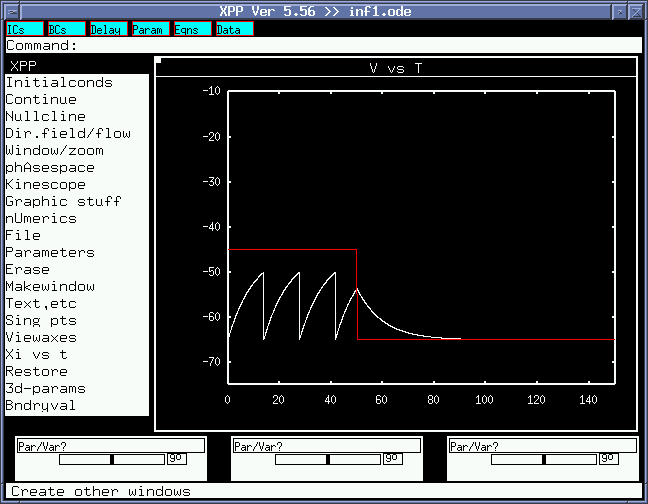
Once you have a window like below (without the plots),
press [i] and [g] in sequence,and you'll see the result. There are two traces, one is the membrane voltage (white), and the other is the steady-state voltage (red). The input was a step input of amplitude 2.0nA, duration 50ms. Note that your threshold should be below the steady-state in order to make the neuron to fire. When the input turns off (I=0), the steady state tends to the resting membrane potential.
Quitting
To quit from the program,
press [f] and [q] and [y] in sequence.
Clearning the plot
To clear the plot,
press [e].
Interacting with XPPAUT: Parameter adjustment
There are several buttons on top of the xppaut window:
Click on the [Param] button and you'll be able to change simulation parameters interactively.
For example, change Vthresh from -50 to -40, and click [Ok] in the parameters window. Then go to the main window and press [e] to clear the plot and then [i] [g] to integrate with the new parameter. You will see that the neuron does not fire this time, since the steady state is below the threshold.
Interacting with XPPAUT: Data
Another useful button is the [Data] button, which allows you to view the
actual numerical data for each dynamic variable, and save the whole thing
into a text file.
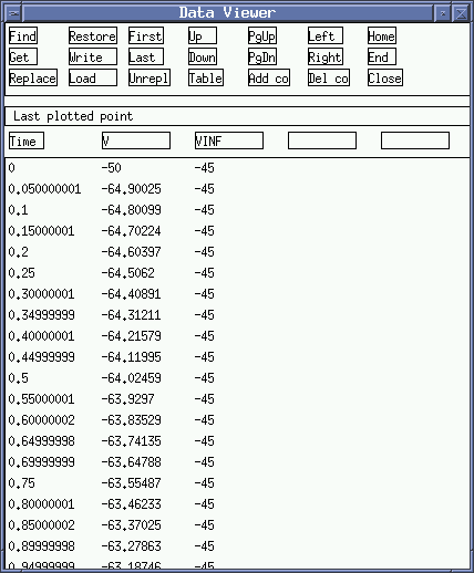
You can see that there are three columns, each representing time, V, and Vinf. Clicking on [Write] (2nd row, 2nd column) will allow you to save the data to a file.
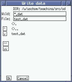
Change the filename to whatever you desire, and click [Ok] to save. You can then use your favorite plotting program to plot the data.
XPPAUT script
The complete file is shown below. There are five sections, parameters,
input, model ODE, simulation configuration, and plotting.
The comments below are self-explanatory, so take a careful look before you
begin. The "#" character is used for comments, so you can selectively
comment out and uncomment parts of the code (especially in section 2. Input)
and press [i] [g].
There are three important lines:
This line sets the initial value of the variable V. Without this, [i] [g] won't work.
This is the heart of the simulation. Note that tau was moved to the right.
This is the spike generation mechanism. When (V-Vthresh) becomes zero, the expression in the braces {V=Erest} gets evaluated.
############################################################################
# Integrate-and-Fire model
# From Dayan and Abbott (2001), section 5.4.
# Parameters are from Fig 5.5.
#
# Written in xppaut by Yoonsuck Choe http://faculty.cs.tamu.edu/choe
# Tue Feb 20 09:36:35 CST 2007
############################################################################

#########################################
# 1. parameters
#########################################

# capacitance: uF
param C=1.0

# resistance : Mohm
param R=10.0

# spike threshold: mV
param Vthresh=-50

# resting membrane potential: mV
param Erest=-65

########################################
# 2. Input: try commenting out different options below.
########################################
#
# 1. constant current: nA
#  I=2.0

# 2. A sinusoidal input (function of t): nA
# I=sin(t/5.0)+2.0

# 3. A step input (heav is the Heaviside step function): nA
  I=heav(-t+50)*2.0

# time constant = R*C: ms
# - to use an expression, you need to define this as a variable rather
#   than a parameter (no "param")
tau=R*C

#########################################
# 3. Model ODE
#########################################
init V=-50

dV/dt=((Erest-V)+R*I)/tau

# reset condition: when (V-theta)=0, the part in {...} gets evaluated.
global 1 (V-Vthresh) {V=Erest}

#########################################
# 4. Simulation configuration
#########################################

# simulation duration
@ total=150

########################################
# 5. Plotting
########################################

# auxiliary variables for plotting
#
# This plots V_infinity, the steady state voltage given a constant input I
aux Vinf=Erest+R*I

# number of plots
@ nplot=2

# designate variables to plot (define yp2, yp3, etc. for 2nd, 3rd plots, etc.)
@ yp1=V
@ yp2=Vinf

# plotting range
@ xlo=0,xhi=150
@ ylo=-75.0,yhi=-10

done
Use these parameters, which are not explicitly stated in the textbook: C=0.3, R_m=90.0, r_m=45.0, Delta_gsra=0.06. You may also use a constant input I=2.0. Don't forget to do {gsra = gsra+Delta_gsra} when a spike occurs (use the global statement).
Run the following experiments and report your results. First, predict what will happen before you run the experiment, and give a reason why you think it will be that way. Then run it, confirming/disproving your insight. Report what you learned.
Try these experiments and report the results: